10 Chi-Square Test

The Chi-Square Test applies to nominal/categorical variables. It has two forms:

A one-way classification to estimate how close an observed distribution is to an expected distribution. This type of test is called a goodness-of-fit test.
A two-way classification to estimate whether two variables from the same population are related or not. This type of test is called a contingency test or test of independence.

The dataset described below will be used to exemplify both types of analyses. It contains all hospital discharges in New York State in 1993 (12,844 records) for patients admitted with an Acute Myocardial Infarction (heart attack) who did not have surgery. The data is defined as shown in Table 10.1.

Table 10.1: Variables in the heart attack data set

Variable	Explanation
age	Patient age in years
gender	Patient’s gender, coded M for males and F for females
diagnosis	Code based on ICD classification
drg	Diagnosis Related Group (121 - with complications who did not die; 122 - without complications who did not die; 123 - patients who died)
los	Hospital length of stay
died	1 if the patient died in the hospital; 0 if not
charges	$ amount of hospital charges

Let’s take a look at how the data looks like by listing the first few rows of the dataset (Table 10.2).

Table 10.2: First few rows of the heart attack data set

diagnosis	gender	drg	charges	los	age
41041	F	122	4752	10	79
41041	F	122	3941	6	34
41091	F	122	3657	5	76
41081	F	122	1481	2	80
41091	M	122	1681	1	55
41091	M	121	6379	9	84

10.1 Goodness-of-Fit Test

Looks at a single categorical variable from a population and attempts to assess how close to or consistent with a hypothesized distribution the actual distribution of that variable is.

Null hypothesis (H₀): The data follows the theoretical distribution.

Before running the analysis, let’s look at a basic descriptive statistic, frequency analysis.

Table 10.3: Gender variable frequencies

Gender	Freq
F	5065
M	7779

Running the chi-square goodness-of-fit test for the gender variable will attempt to test for equal counts in every cell of the design.


    Chi-squared test for given probabilities

data:  table(my.ha$gender)
X-squared = 570, df = 1, p-value <2e-16

Given the small p-value, the null hypothesis can be rejected and it can be considered that the alternative is true.

Example of how to write it up:

The null hypothesis stating that patients are equally distributed across genders, $\chi^{2}(df = 1) = 573.48, p < 0.001$ is rejected. Therefore, there are significant differences between the expected number of patients for each gender and the observed number.

Observed frequencies can help explain the direction of the relationship for the possible underlying explanation or reason. This explanation can be added to the text if relevant for the study.

10.2 Test of Independence

In this case the Chi-Square Test is used to determine if a significant relationship exists between two categorical variables. The test compares the frequency of each category of one of the variables to the frequency for each of the categories of the other variable.

In this example we will try to find if there number of patients deaths is in some way related to their gender. Therefore, we will be testing the null hypothesis:

The null hypothesis (H₀): There is no relationship between gender and the patient dying in the hospital.

Let’s look at some cell counts first. An idea about how these look like will be useful later when compared with expected cell counts computed from the statistical test.

Table 10.4: Gender count and Died (0 = no, 1 = yes) by gender variable counts

	0	1
F	4298	767
M	7136	643

Now let’s run the test:


    Pearson's Chi-squared test with Yates' continuity correction

data:  table(my.ha$gender, my.ha$died)
X-squared = 150, df = 1, p-value <2e-16

The obtained p-value < .05 indicates that the null hypothesis (indicating independence) can be safely rejected and the alternative hypothesis (indicating the existence of a relationship between gender and died) should be accepted.

If the null hypothesis were true, the expected counts are shown in Table 10.5, compared to the observed frequencies shown in Table 10.4.

Table 10.5: Expected frequencies

	0	1
F	4509	556
M	6925	854

A mosaic plot (Figure 10.1) can help visualize the relative cell sizes.

Figure 10.1: Mosaic plot of gender vs. age

Now let’s look at a chi-square analysis when at least one of the variables has more than one level. In this case we will be using the drg variable8989 The drg (Diagnosis Related Group) has three levels: 121 - with complications who did not die; 122 - without complications who did not die; 123 - patients who died..

The cell counts in this case are shown in Table 10.6.

Table 10.6: Gender count and Diagnostic Related Group variable counts

	121	122	123
F	2328	1970	767
M	3059	4077	643

Running the test returns the results shown below.


    Pearson's Chi-squared test

data:  table(my.ha$gender, my.ha$drg)
X-squared = 280, df = 2, p-value <2e-16

And the mosaic plot is presented in Figure 10.2.

Figure 10.2: Relationship between Gender and Diagnostic Related Group (drg)

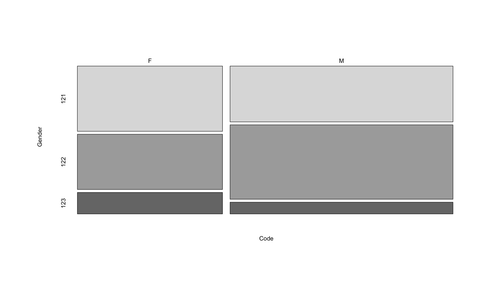
Table 10.7 shows the expected frequencies when the null hypothesis (H₀) is true. Compare them with the observed frequencies shown in Table 10.6.

Table 10.7: Expected frequencies

	121	122	123
F	2124	2385	556
M	3263	3662	854

Example of how to write it up:

The null hypothesis stating that there is no relationship between gender and diagnosis related group classification, $\chi^{2}(df = 2) = 283.43, p < 0.001$ is rejected. Therefore, the differences between the number of males and females in the different diagnosis related group are significant.