13 MANOVA: Multiple Analysis of Variance
Used to compare means of multiple criterion (dependent) variables between two or more groups defined by the predictor (independent) variable. A different data set is going to be used as an example for this analysis. To better understand the example, the study scenario is introduced below.
A research to study the effect of race stereotypical crimes was conducted with 105 participants. Three identical versions of a scenario about a crime, referencing one of three ethnicities (African-American, Hispanic, Caucasian) were randomly presented to the participants. The study measured92 Column labels are: ethnicity, punish, repeats, and dispos.:
- Dependent variables:
- Perceived level of punishment (“punish”);
- Perceived likelihood of committing the same crime again (“repeat”);
- Perceived likelihood that the reason the defendant committed the crime was due to his/her character, or disposition (“dispos”);
- Independent variable:
- Ethnicity93 Labels used for the independent variable, ethnicity, are: 0 = African-American, 1 = Hispanic, and 2 = Caucasian..
Null Hypothesis (H0): In the population, there is no difference in perceived level of punishment to be administered to the defendant, perceived likelihood the defendant will commit the same crime again, and the perceive likelihood that the reason the defendant committed the crime was due to his or her character for African-American, Hispanic, and Caucasian ethnicities.
The analysis is a one-way MANOVA for a between groups design.
13.1 Outliers
To determine whether the data set has outliers let’s use a graphical representation. The primary plot represents the ordered squared robust Mahalanobis distances against the empirical distribution function \(MD^2_i\). Of the three additional graphs the first shows the data, the second attempts to highlight potential outliers as detected using the \(chisq_p\) distribution, and the third presenting the outliers by the adjusted quantile (Filzmoser, Garret, and Reimann 2005Filzmoser, P., R.G. Garret, and C. Reimann. 2005. “Multivariate Outlier Detection in Exploration Geochemistry.” Computers and Geosciences, no. 31: 579–87.).
Projection to the first and second robust principal components.
Proportion of total variation (explained variance): 0.9381
Figure 13.1: Outliers in the dataset
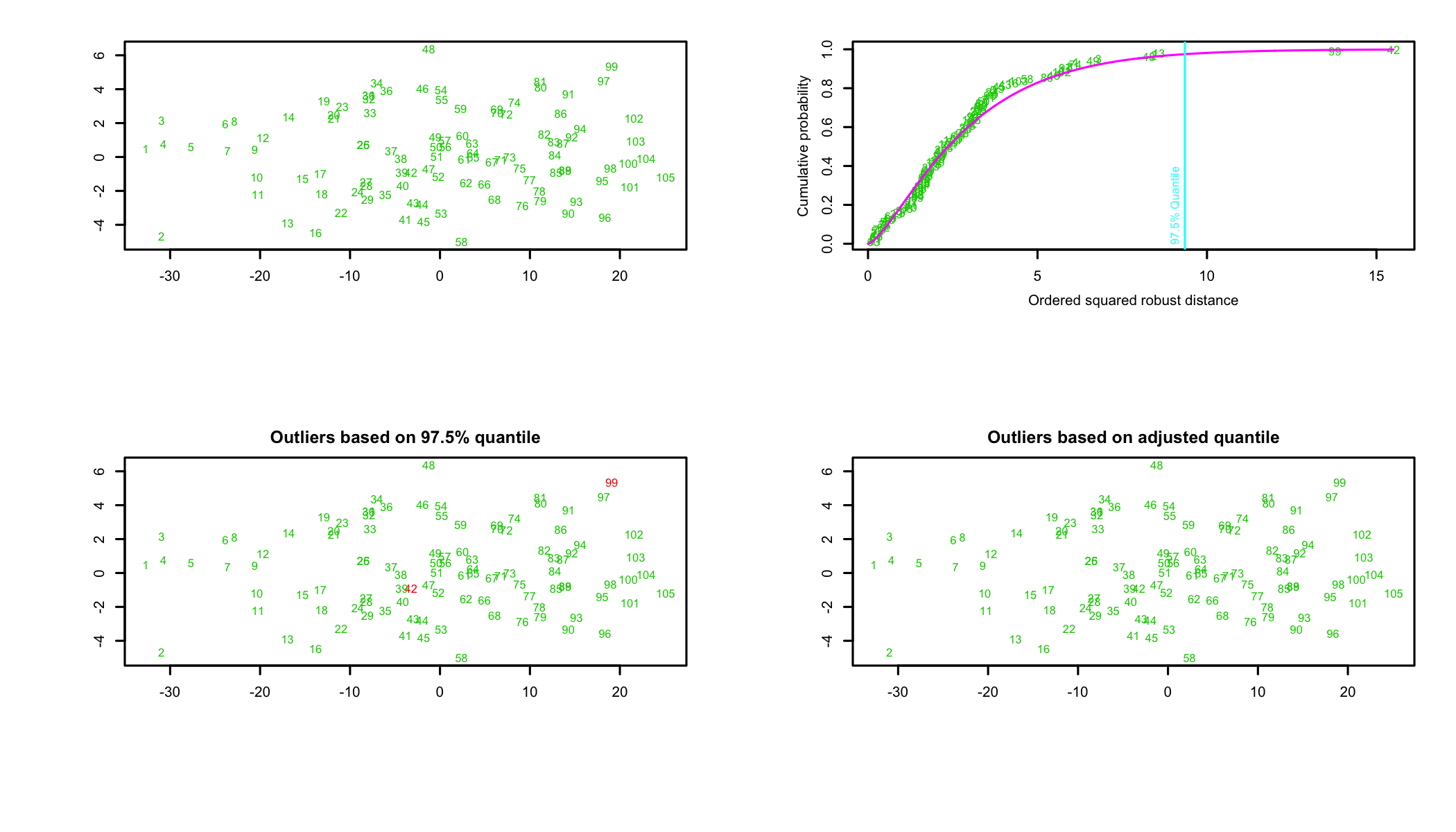
Two of plots in Figure 13.1 show two cases, 42 and 99, as potential outliers while the third, the outliers based on adjusted quantiles, suggests that the dataset has no outliers. In this case, the decision is left to the researcher. Each outlier should be analyzed individually and a decision should be made if it is to be removed or not. The criteria used for such decisions can range from theoretical necessity of including the possible outliers in the analysis to the point highlighted as outlier to be a valid data point based on an in-depth analysis of the data. In this example, because the analysis does not conclusively highlight the two cases as outliers, they will not be removed94 A more extensive analysis, outside the scope of this chapter, focused on the two possible outliers conducted on the dataset led to the same conclusion..
13.2 Assumptions
Before conducting the analysis, assumptions of normality, homogeneity of covariances, homogeneity of variances, and independence of observations need to be tested.
Summary statistics including skewness and kurtosis95 In the output, X1 refers to the dependent variable being analyzed: punish, repeats, dispos..
DV: punish
 Descriptive statistics by group
group: African-American
   vars  n  mean    sd median trimmed   mad min max range skew kurtosis
X1    1 24 49.33 11.09   50.5   49.25 13.34  30  71    41 0.08    -1.13
     se
X1 2.26
--------------------------------------------------------
group: Hispanic
   vars  n  mean    sd median trimmed   mad min max range  skew kurtosis
X1    1 26 57.77 14.71   60.5   58.64 16.31  28  79    51 -0.55    -0.68
     se
X1 2.89
--------------------------------------------------------
group: Caucasian
   vars  n  mean    sd median trimmed   mad min max range  skew kurtosis
X1    1 55 65.89 10.54     67   65.91 11.86  46  85    39 -0.04    -1.13
     se
X1 1.42
The output shows various basic statistics, such as the mean of the variable, its median, mean, and so forth. Of interest here is the reported swkewness and kurtosis. The values suggest a normally distributed dataset for the punish variable for each of the three ethnic groups. A similar analysis is performed below for the two other variables in the analysis, repeats and dispos. In each case, the skewness and kurtosis are well within the limits.
DV: repeats
 Descriptive statistics by group
group: African-American
   vars  n  mean   sd median trimmed  mad min max range skew kurtosis   se
X1    1 24 24.12 2.17     24   24.05 2.97  21  28     7 0.26    -1.24 0.44
--------------------------------------------------------
group: Hispanic
   vars  n  mean   sd median trimmed  mad min max range skew kurtosis   se
X1    1 26 24.23 2.25     24   24.32 2.97  20  28     8 -0.3       -1 0.44
--------------------------------------------------------
group: Caucasian
   vars  n  mean   sd median trimmed  mad min max range  skew kurtosis
X1    1 55 25.53 1.99     26   25.58 1.48  21  29     8 -0.21    -0.62
     se
X1 0.27
DV: dispos
 Descriptive statistics by group
group: African-American
   vars  n mean   sd median trimmed  mad min max range skew kurtosis   se
X1    1 24   23 2.27     23    22.9 2.97  20  28     8 0.26    -1.03 0.46
--------------------------------------------------------
group: Hispanic
   vars  n  mean   sd median trimmed  mad min max range  skew kurtosis  se
X1    1 26 23.46 2.04     24   23.45 1.48  20  27     7 -0.15     -1.1 0.4
--------------------------------------------------------
group: Caucasian
   vars  n  mean   sd median trimmed  mad min max range  skew kurtosis
X1    1 55 24.91 2.47     25   25.07 2.97  20  29     9 -0.44    -0.84
     se
X1 0.33
13.2.1 Visual Evaluation of Data Normality
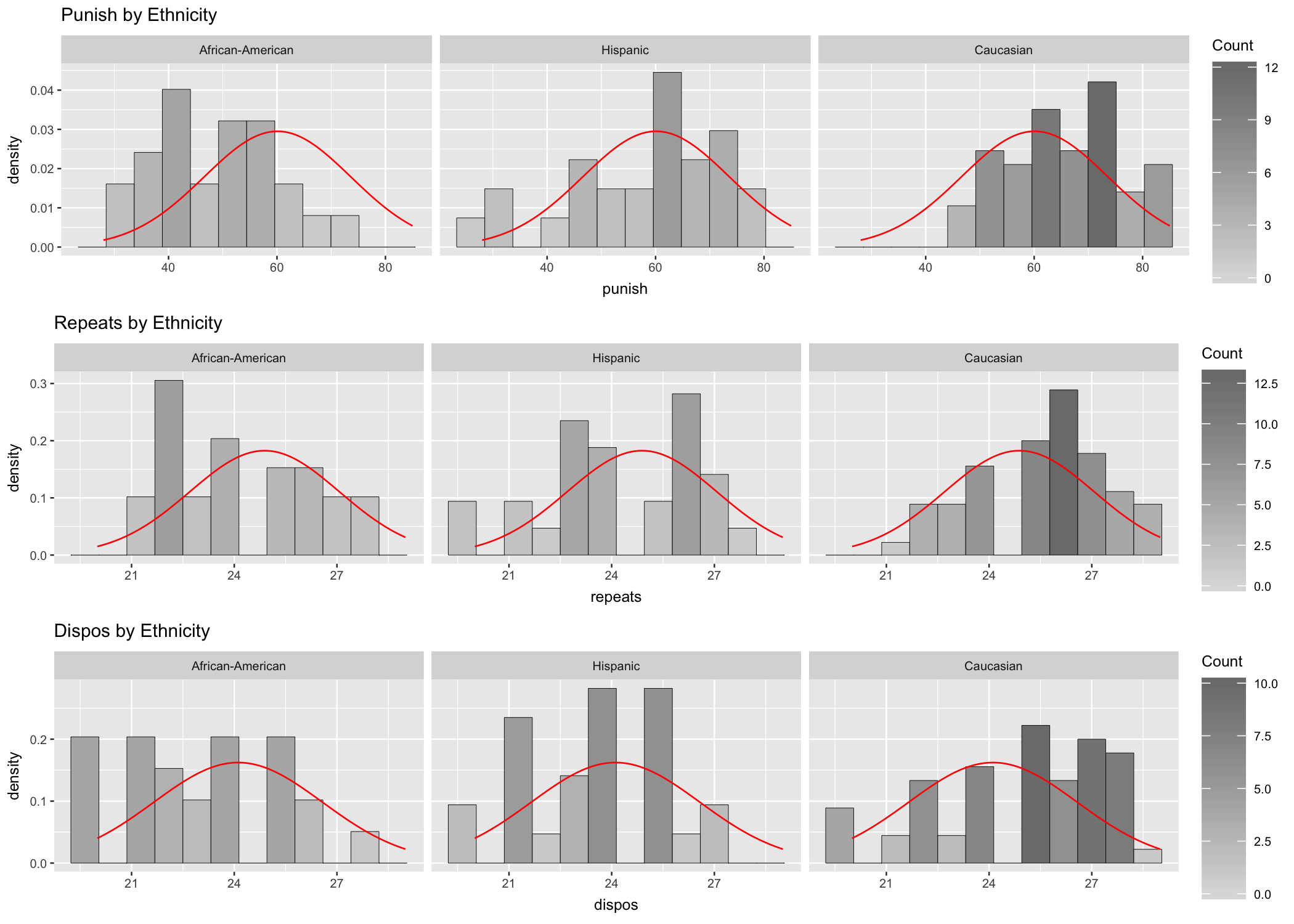
For analysis we produce the appropriate qq-plots (Fig. 13.2) and histograms (Fig. 13.3). A cursory review of the plots seem to suggest that departure from normality may exist, at least for some of the groups. Observe the top-left plot in Fig. 13.2 (level of punishment for African Americans). The points representing the data align neatly along the diagonal line, which suggests that data is normally distributed. Other plots show an S-shaped distribution of the data point alongside the diagonal, which suggests departures from normality. The histograms in Fig. 13.3 seem to suggest similar possible departures from normality. In this situation further analysis is necessary to determine if the assumption of normality is met.
Figure 13.2: qq-plots
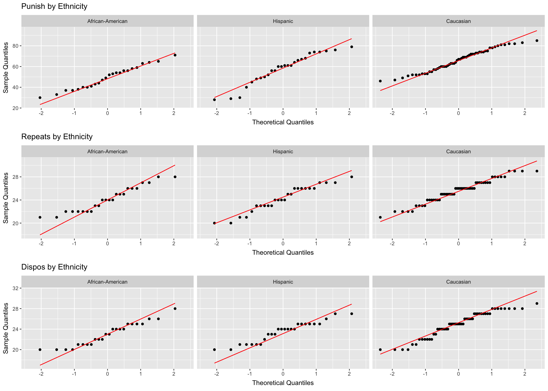
Figure 13.3: Histograms
13.2.2 Shapiro-Wilk Test of Normality
Shapiro-Wilks is used to test normality of data for each subgroup. Table 13.1 combines summary statistics and the Shapiro-Wilk test for the design groups.
Table 13.1: Shapiro-Wilk test of normality
| Dependent Variable | Ethnicity | Statistic | df | Sig. |
|---|---|---|---|---|
| Level of punishment | African American | 0.97 | 25 | 0.703 |
| Hispanic | 0.94 | 26 | 0.110 | |
| Caucasian | 0.97 | 55 | 0.130 | |
| Potential to repeat | African American | 0.93 | 25 | 0.101 |
| Hispanic | 0.95 | 26 | 0.183 | |
| Caucasian | 0.96 | 55 | 0.087 | |
| Natural disposition | African American | 0.95 | 25 | 0.132 |
| Hispanic | 0.93 | 26 | 0.079 | |
| Caucasian | 0.94 | 55 | 0.005 |
Table 13.1 shows that most of the cells (with the exception of the last line in the table), have a low significance level that may be indicative of the fact that even if the Shapiro-Wilk test suggests that the data is within the normality conditions, its distribution in each cell is not as close to the normal distribution as one would want it to be.
13.2.3 Multivariate Normality
The homogeneity of covariances can be analyzed using Box’s test. With an observed significance of .2 the null hypothesis, stating that the covariance matrices of the dependent variables are equal across groups, is accepted.
    Box's M-test for Homogeneity of Covariance Matrices

data:  variables
Chi-Sq (approx.) = 17, df = 12, p-value = 0.2
Levene’s test of equality of error variances:
Level of PuhishmentLevene's Test for Homogeneity of Variance (center = median)
Df F value Pr(>F)
group 2 1.14 0.32
102 Potential to RepeatLevene's Test for Homogeneity of Variance (center = median)
Df F value Pr(>F)
group 2 0.55 0.58
102 Natural DispositionLevene's Test for Homogeneity of Variance (center = median)
Df F value Pr(>F)
group 2 0.65 0.52
102 Levene’s tests of equality of variances shows that the error variance of all three dependent variables is equal across groups.
One last assumption to consider - independence of observations - seems reasonable because the treatments were administered individually.
13.3 The MANOVA Test
Now that the assumptions have been tested and the results show that the data set is appropriate for analysis, run the MANOVA test.
           Df Wilks approx F num Df den Df  Pr(>F)
ethnicity   2 0.731     5.66      6    200 1.9e-05 ***
Residuals 102
---
Signif. codes:  0 '***' 0.001 '**' 0.01 '*' 0.05 '.' 0.1 ' ' 1
To better understand what the results tell us let’s look at the effect size (\(\eta^{2}\)). The threshold values for evaluating the effect size (partial \(\eta^{2}\)) are .01 for small effect size, .08 for moderate effect size, and .14 for large effect size. Any value below .01 indicates no effect.
           eta^2
ethnicity 0.1452
The write-up may look like below:
A significance value p < .001, together with F(6,200) = 5.66, p < .05 and a large effect size, suggested by a partial \(\eta^{2}= .145 (> .14)\) for the multivariate tests, indicate a significant multivariate effect of ethnicity on the three dependent variables. Therefore, the null hypothesis (H0) can be rejected.
13.3.1 Univariate Statistics
While the MANOVA multivariate statistics looks the dependent variables together, it may also be of interest for researchers to look how ethnicity affects the behavior of each dependent variable individually in multivariate context.
 Response 1 :
             Df Sum Sq Mean Sq F value Pr(>F)
ethnicity     2   4768    2384    17.1  4e-07 ***
Residuals   102  14243     140
---
Signif. codes:  0 '***' 0.001 '**' 0.01 '*' 0.05 '.' 0.1 ' ' 1

 Response 2 :
             Df Sum Sq Mean Sq F value Pr(>F)
ethnicity     2     48    23.8    5.42 0.0058 **
Residuals   102    449     4.4
---
Signif. codes:  0 '***' 0.001 '**' 0.01 '*' 0.05 '.' 0.1 ' ' 1

 Response 3 :
             Df Sum Sq Mean Sq F value Pr(>F)
ethnicity     2     76    37.8    6.97 0.0014 **
Residuals   102    553     5.4
---
Signif. codes:  0 '***' 0.001 '**' 0.01 '*' 0.05 '.' 0.1 ' ' 1
Level of Punishment Partial eta^2
ethnicity 0.2508
Residuals NAPotential to Repeat Partial eta^2
ethnicity 0.09601
Residuals NANatural Disposition Partial eta^2
ethnicity 0.1203
Residuals NAThe univariate statistics analysis show that ethnicity has univariate effects on all three dependent variables as the significance p values for all three dependent variables are < .01. For effect size, ethnicity shows a large effect size on the Level of punishment (punish) (partial \(\eta^{2}\) = .251), and moderate effect size on the other two dependent variables, Potential to repeat (repeat) and Natural disposition (dispos), which have values of partial \(\eta^{2} = .096\) and .12 respectively.