14 ANCOVA: Analysis of Covariance
At a glance
- Question
- Do the means of two or more groups differ after controlling for a covariate?
- Design
- Two or more independent groups, ideally formed by random assignment; the covariate measured before the treatment
- Dependent variable
- Interval or ratio
- Independent variable
- Nominal, two or more levels
- Covariate
- Continuous, related to the DV, chosen before the study
- Assumptions
-
- Independent observations
- Normality of the residuals and equal variances in the groups
- A linear relationship between the covariate and the DV in each group
- Homogeneity of regression slopes: no covariate \times group interaction
- Null hypothesis
- The adjusted population means are equal
- Test statistic
- F for the groups, after the covariate
- Effect size
- Partial \eta^{2}: .01 small, .06 medium, .14 large
- If conditions fail
-
- The regression slopes differ between the groups → A regression with an interaction
- Include in the write-up
-
- The assumption checks, including the covariate \\times group interaction
- F for the covariate, and F(df1, df2) = …, p = …, \eta^{2}_{p} for the groups
- The adjusted means, and the pairwise comparisons
Used to compare the means of a dependent (criterion) variable between two or more groups defined by an independent (predictor) variable, while controlling for one or more continuous variables, called covariates. A covariate is a variable that is related to the dependent variable but is not of interest in itself11 Typical covariates are the scores of the participants on a pretest, their prior knowledge of a subject, or their age..
1 Typical covariates are the scores of the participants on a pretest, their prior knowledge of a subject, or their age.
The ANCOVA combines the one-way ANOVA with regression. Its model includes both the groups and the covariate:
\hat{Y}_i = b_0 + b_1 D_{1i} + \dots + b_{k-1} D_{(k-1)i} + b_k C_i
where the D variables code the groups and C is the covariate. Including the covariate in the analysis has two benefits:
- It reduces the error variance. Part of the differences between the participants within each group is due to the covariate. Removing it from the error term makes the test of the groups more powerful;
- It adjusts the group means. The groups are compared as if all participants had the same value of the covariate, which removes the part of the group differences that is due to the covariate.
The first benefit is the main reason to use ANCOVA in randomized experiments. The second needs more care. When the participants are randomly assigned to the groups, the groups differ on the covariate only by chance, and the adjustment is small. When the groups already existed before the study, for example classes taught by different teachers, they may differ on the covariate for reasons that are related to the groups themselves. In that case the adjustment does not make the groups comparable, and the results cannot be interpreted as if they had been22 This is one of the most common misuses of ANCOVA. Controlling for a covariate does not turn existing groups into randomly assigned ones. See also A Few Words About Causality..
2 This is one of the most common misuses of ANCOVA. Controlling for a covariate does not turn existing groups into randomly assigned ones. See also A Few Words About Causality.
14.1 The Theory
14.1.1 Partitioning the Variance
The ANCOVA removes the variability explained by the covariate before the groups are tested. The total sum of squares is divided into three parts:
SS_{T} = SS_{C} + SS_{M(adj)} + SS_{R(adj)}
where SS_{C} is the part explained by the covariate, SS_{M(adj)} the part explained by the groups after the covariate has been taken into account, and SS_{R(adj)} the part left unexplained33 The covariate uses one degree of freedom, which is taken from the residual.. With k groups and N participants, the groups are tested with:
3 The covariate uses one degree of freedom, which is taken from the residual.
F = \frac{SS_{M(adj)} / (k - 1)}{SS_{R(adj)} / (N - k - 1)}
The covariate has its own F test, with 1 and N - k - 1 degrees of freedom. A covariate that is not related to the dependent variable only costs a degree of freedom. For this reason the covariates are chosen before the study, from theory and prior research, as variables known to be related to the dependent variable. Once chosen, a covariate is kept in the model even if its own F test is not significant44 Dropping it after seeing the results is a choice made from the data, which makes the p-value of the groups less trustworthy..
4 Dropping it after seeing the results is a choice made from the data, which makes the p-value of the groups less trustworthy.
14.1.2 Adjusted Means
The adjusted means are the group means predicted by the model for a participant with the mean value of the covariate. When the covariate is positively related to the dependent variable, as a pretest usually is, a group with a higher mean on the covariate than the other groups has an adjusted mean on the dependent variable lower than its observed mean, and the other way around. With a negative relationship, the adjustment goes in the opposite direction. The groups are compared on their adjusted means.
14.1.3 Effect Size
As in a factorial ANOVA, the effect size of the groups is the partial eta squared, the variability explained by the groups relative to that variability plus the error:
\eta^{2}_{p} = \frac{SS_{M(adj)}}{SS_{M(adj)} + SS_{R(adj)}}
It is read with the usual guidelines: .01 small, .06 medium, and .14 or more large.
14.2 Assumptions
The ANCOVA has the assumptions of the one-way ANOVA, applied to the residuals of the model, and three more that concern the covariate:
- Independence of observations
- Usually ensured by the design of the study;
- Violated when the participants influence each other or are measured more than once.
- Normality of residuals and homogeneity of variances
- Detected using a q-q plot and a test of normality of the residuals, and Levene’s test across the groups;
- Violated as in the one-way ANOVA.
- Linear relationship between the covariate and the dependent variable, in each group
- Detected using a scatter plot of the dependent variable against the covariate, by group;
- Violated when the points follow a curve.
- Independence of the covariate and the groups
- Ensured by the design: random assignment to the groups, and a covariate measured before the treatment;
- Detected by comparing the groups on the covariate with a one-way ANOVA, as a description. A non-significant difference does not prove that the groups are the same on the covariate;
- Violated when the groups differ on the covariate for reasons related to the groups themselves, as with groups that existed before the study. In a randomized study, a chance difference is not a violation: it is what the adjustment corrects. A covariate measured after the treatment is not independent of it55 A covariate measured after the treatment may itself have been changed by it. Controlling for it would then remove part of the effect of the treatment..
5 A covariate measured after the treatment may itself have been changed by it. Controlling for it would then remove part of the effect of the treatment.
- Homogeneity of regression slopes
- Detected by testing the interaction between the covariate and the groups;
- Violated when the interaction is significant: the relationship between the covariate and the dependent variable is not the same in all groups. In that case a single adjustment does not fit all groups, and the interaction between the covariate and the groups should be studied as such, with a regression model.
14.3 The Study
A statistics department developed three versions of an online module that introduces students to hypothesis testing: a Text version, with readings and worked examples, a Video version, with short recorded lectures, and an Interactive version, with simulations the students could manipulate. Sixty students were randomly assigned to one of the three versions, 20 to each. Before the module, the students took a short math background test (pretest, scored from 0 to 50). At the end of it, they took a quiz on hypothesis testing (quiz, scored from 0 to 100). The question asked is: Does the version of the module make a difference in what the students learned? The data set66 Column labels are: student, version, pretest, and quiz. was made up for this example. The first few rows of the data set are shown in Table 14.1.
6 Column labels are: student, version, pretest, and quiz.
| Student | Version | Pretest | Quiz |
|---|---|---|---|
| 1 | Text | 32 | 70 |
| 2 | Text | 31 | 72 |
| 3 | Text | 40 | 88 |
| 4 | Text | 21 | 63 |
| 5 | Text | 20 | 44 |
| 6 | Text | 34 | 75 |
The math background of the students is expected to affect their quiz scores, whatever version of the module they used. It is not of interest in itself, but it adds variability to the quiz scores that has nothing to do with the module. It is therefore used as a covariate.
Hypotheses.
- Null hypothesis (H0): In the population, once the math background is taken into account, the mean quiz score is the same for the three versions of the module.
- Alternative hypothesis (H1): At least one version leads to a different adjusted mean quiz score.
Decision criteria. The significance level is set at \alpha = .05. With 3 groups, one covariate, and 60 students, the test of the groups has 2 and 60 - 3 - 1 = 56 degrees of freedom. H0 is rejected if the p-value is smaller than \alpha. The effect size is \eta^{2}_{p}. A significant result is followed up with pairwise comparisons of the adjusted means, with a Bonferroni correction.
14.3.1 Describing the Groups
| Version | n | Pretest M | Pretest SD | Quiz M | Quiz SD |
|---|---|---|---|---|---|
| Text | 20 | 29.40 | 6.73 | 68.70 | 11.59 |
| Video | 20 | 29.60 | 7.45 | 70.35 | 10.51 |
| Interactive | 20 | 30.10 | 8.43 | 75.75 | 14.13 |
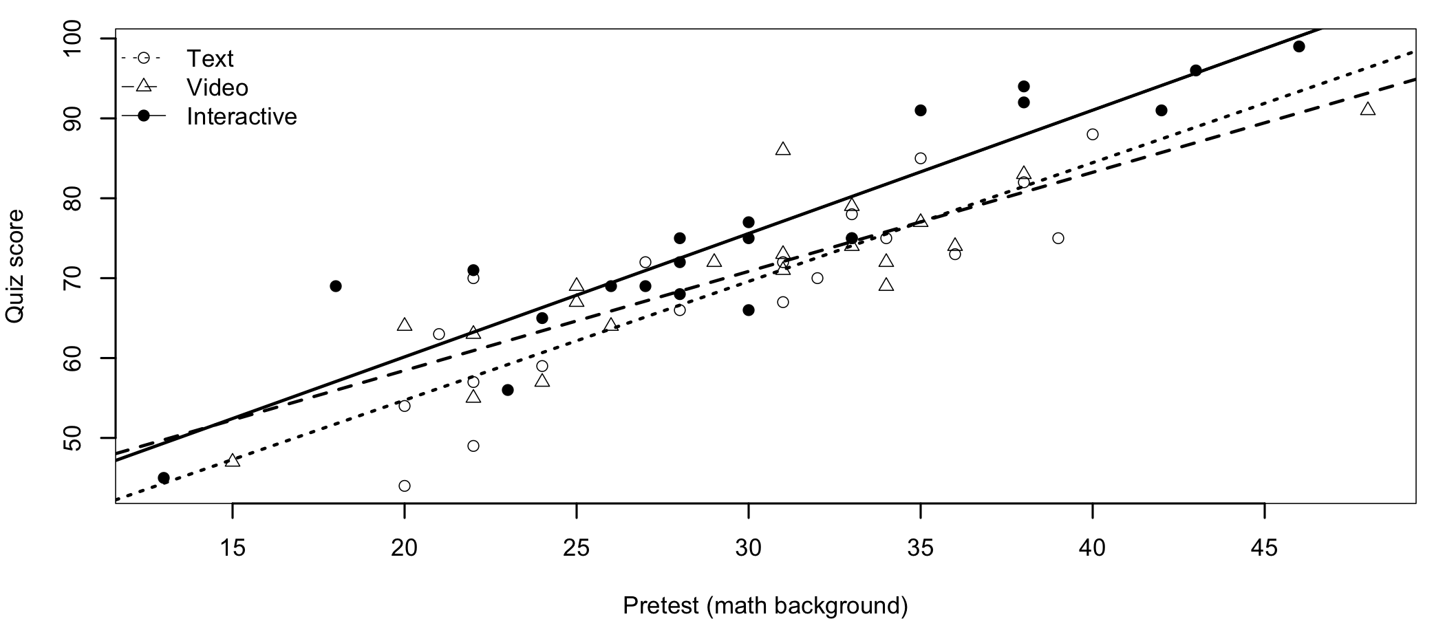
The three groups have almost the same mean on the pretest (Table 14.2), as expected from random assignment. On the quiz, the students who used the interactive version obtained the highest mean, but the standard deviations are large compared with the differences between the means. Figure 14.1 shows why: the quiz scores depend strongly on the math background of the students (r = 0.87). Within each version, students with a stronger background scored much higher than those with a weaker one. The three lines are roughly parallel, and the line of the interactive version is above the other two.
14.3.2 The ANOVA Without the Covariate
To see what the covariate brings to the analysis, let’s first run a one-way ANOVA on the quiz scores, ignoring the pretest.
            Df Sum Sq Mean Sq F value Pr(>F)
version      2    544   271.9   1.835  0.169
Residuals   57   8446   148.2
The ANOVA finds no significant difference between the three versions, F(2, 57) = 1.84, p = .169. The differences between the versions are hidden by the large differences between the students within each version.
14.3.3 Checking the Assumptions
The independence of observations is supported by the design: the students were randomly assigned to the versions and worked on the module on their own. The linearity of the relationship between the pretest and the quiz is visible in Figure 14.1, in all three groups.
Independence of the covariate and the groups. The pretest was taken before the module, and the groups are compared on it with a one-way ANOVA:
            Df Sum Sq Mean Sq F value Pr(>F)
version      2    5.2   2.600  0.0454 0.9557
Residuals   57 3265.4  57.288
The groups do not differ significantly on the pretest, F(2, 57) = 0.05, p = .956.
Homogeneity of regression slopes. The model is fitted with the interaction between the covariate and the groups. The assumption is met if the interaction is not significant.
Anova Table (Type III tests)

Response: quiz
                Sum Sq Df  F value    Pr(>F)
(Intercept)     2910.4  1  92.2103 2.816e-13 ***
pretest         6397.5  1 202.6952 < 2.2e-16 ***
version           38.8  2   0.6149    0.5444
pretest:version   58.5  2   0.9267    0.4021
Residuals       1704.4 54
---
Signif. codes:  0 '***' 0.001 '**' 0.01 '*' 0.05 '.' 0.1 ' ' 1
The interaction is not significant, F(2, 54) = 0.93, p = .402. There is no evidence that the relationship between the pretest and the quiz differs between the three groups.
Normality of residuals and homogeneity of variances. These are checked on the ANCOVA model, without the interaction.
    Shapiro-Wilk normality test

data:  resid(my.anc)
W = 0.98641, p-value = 0.7429
Levene's Test for Homogeneity of Variance (center = mean)
Df F value Pr(>F)
group 2 0.0764 0.9265
57 The residuals do not depart significantly from normality (Shapiro-Wilk p = .743), and their variances do not differ significantly across the groups (Levene’s test, p = .927).
No assumption is clearly violated, so we can proceed with the analysis.
14.3.4 The ANCOVA Test
Anova Table (Type III tests)

Response: quiz
            Sum Sq Df  F value    Pr(>F)
(Intercept) 2954.5  1  93.8544 1.425e-13 ***
pretest     6683.6  1 212.3173 < 2.2e-16 ***
version      402.0  2   6.3846  0.003179 **
Residuals   1762.9 56
---
Signif. codes:  0 '***' 0.001 '**' 0.01 '*' 0.05 '.' 0.1 ' ' 1
Decision. Once the math background is taken into account, the version of the module has a significant effect on the quiz scores, F(2, 56) = 6.38, p = .003. The null hypothesis is rejected and the alternative hypothesis accepted. The covariate is also significant, F(1, 56) = 212.32, p < .001, which confirms that it belongs in the model.
Effect size. \eta^{2}_{p} = 0.19 for the version of the module, a large effect.
Why does the ANCOVA find a difference that the ANOVA did not? The answer is in the error term. In the ANOVA, the residual sum of squares was 8446.5. In the ANCOVA, after the pretest has explained its part, it is only 1762.9, 79% less. The differences between the versions are about the same in both analyses, but they are compared with much less noise.
14.3.5 Adjusted Means and Pairwise Comparisons
 version     emmean   SE df lower.CL upper.CL
 Text          69.1 1.25 56     66.6     71.6
 Video         70.5 1.25 56     68.0     73.0
 Interactive   75.2 1.26 56     72.7     77.7

Confidence level used: 0.95
contrast estimate SE df t.ratio p.value
Text - Video -1.36 1.77 56 -0.769 1.0000
Text - Interactive -6.05 1.78 56 -3.407 0.0037
Video - Interactive -4.68 1.77 56 -2.639 0.0322
P value adjustment: bonferroni method for 3 tests Because the groups had similar pretest scores, the adjusted means (69.13, 70.49, and 75.18) are close to the observed means. The pairwise comparisons, with a Bonferroni correction, show that the students who used the interactive version scored higher than those who used the text version, by 6.05 points, t(56) = 3.41, p = .004, and than those who used the video version, by 4.68 points, t(56) = 2.64, p = .032. The text and video versions did not differ significantly (p = 1.000).
14.3.6 Reporting the Results
| Source | df | SS | MS | F | p | η2p |
|---|---|---|---|---|---|---|
| Pretest (covariate) | 1 | 6683.65 | 6683.65 | 212.32 | < .001 | .79 |
| Version | 2 | 401.97 | 200.98 | 6.38 | .003 | .19 |
| Residuals | 56 | 1762.85 | 31.48 |
Here is an example of how to write up the results in a publication, together with Table 14.3.
A one-way ANCOVA compared the quiz scores of 60 students randomly assigned to three versions of an online statistics module, controlling for their math background (pretest). The groups did not differ significantly on the pretest, p = .956, the relationship between the pretest and the quiz did not differ significantly between the three groups (pretest × version p = .402), and the residuals did not depart significantly from normality (Shapiro-Wilk p = .743), with no significant difference in their variances (Levene’s test p = .927). The pretest was significantly related to the quiz scores, F(1, 56) = 212.32, p < .001. After controlling for the pretest, the version of the module had a significant effect on the quiz scores, F(2, 56) = 6.38, p = .003, η2p = .19. Bonferroni-corrected comparisons of the adjusted means showed that the students who used the interactive version (Madj = 75.18) scored higher than those who used the text (Madj = 69.13, p = .004) or the video version (Madj = 70.49, p = .032), which did not differ from each other.
14.4 Summary
The ANCOVA compares groups while controlling for a covariate, a continuous variable related to the dependent variable. In a randomized experiment, its main benefit is power. In the statistics module study, the ANOVA could not find a difference between the three versions, because the differences in the students’ math background hid it. Once the background was taken into account, the interactive version proved better than the other two.
Of note is the fact that a covariate should be chosen before the data is collected, based on what is known about the dependent variable, and measured before the treatment77 Trying several covariates until one of them makes the result significant is a form of data dredging.. The assumptions of the ANCOVA also need attention: the covariate should be independent of the groups, and its relationship with the dependent variable should be the same in all groups. When the groups differ on the covariate because they existed before the study, the ANCOVA cannot make them equal.
7 Trying several covariates until one of them makes the result significant is a form of data dredging.