9 Normalization, Standardization, and Data Transformation
In statistics the term normalization can have multiple meanings. For example, it can mean to adjust values of variables to be analyzed to a common scale when these variables are measured using different scales. Alternatively, normalization may mean to transform the values of a sample to get it closer to the normal distribution, to fulfill the assumption of normally distributed data underlying many common statistical tests. Or, in other situations, normalization could be an attempt to eliminate the effects of known influences.
Sometimes the term normalization is used interchangeably with the term standardization. While both serve the same general purpose, there is a difference:
- Normalization: intended to scale a variable to a range of values between 0 and 1;
- Standardization (e.g., z-score): intended to transform a variable to have its mean = 0 and SD11 Standard Deviation = 1.
1 Standard Deviation
Some of the processes that fall under the concept of normalization may be called data transformation22 IMPORTANT: A transformed value, such as the log of a value, is hard to interpret and present. Therefore, once the analysis has been performed, the results should be converted back to the original units by applying the reverse of the formula used to transform the data. Of note is the fact that the converted results do not always mean the same thing as the original statistics. The mean of log-transformed data, for example, converts back to the geometric mean, not to the ordinary (arithmetic) mean. See Converting the Results Back.. While all this may be confusing, the process always involves a purposeful conversion of the data of a data set from its current format to a different format. In most situations, the process also involves eliminating the units of measure with the intent of making the comparison easier.
2 IMPORTANT: A transformed value, such as the log of a value, is hard to interpret and present. Therefore, once the analysis has been performed, the results should be converted back to the original units by applying the reverse of the formula used to transform the data. Of note is the fact that the converted results do not always mean the same thing as the original statistics. The mean of log-transformed data, for example, converts back to the geometric mean, not to the ordinary (arithmetic) mean. See Converting the Results Back.
9.1 Scaling/Rescaling
A very simple process which aims to change the spread of the data and/or the position of the data points. The transformation uses a simple linear equation of the form y=a\times x+b, which changes the data’s median, mean (\mu), and standard deviation (\sigma), but leaves unchanged the shape of the distribution and the z-scores33 Because they are calculated as a ratio of the difference between the actual value and the sample’s mean and the sample’s standard deviation. In essence, the z-score indicates how many standard deviations from the mean the data point is..
3 Because they are calculated as a ratio of the difference between the actual value and the sample’s mean and the sample’s standard deviation. In essence, the z-score indicates how many standard deviations from the mean the data point is.
The more common are:
- Range scaling: change the data from one range to another (magnification or reduction)44 Often times done to bring the variables in an analysis to the same scale.. The min-max normalization is a special case that maps the smallest value to 0 and the largest to 1, x' = \frac{x - min}{max - min};
4 Often times done to bring the variables in an analysis to the same scale.
- Mean centering: subtracts the mean of the sample from each data point. The data keeps its spread and shape, but shifts so that its mean becomes 055 Often done to center the analysis on the variation part of the data rather than, for example, a center tendency value.;
5 Often done to center the analysis on the variation part of the data rather than, for example, a center tendency value.
- Standardization: is intended to make data samples comparable. The process does not change the shape of the distribution, only the mean and the standard deviation. The most common method is the z-transform used to convert the data to z-scores, z = \frac{x - \bar{x}}{s}. Also called auto-scaling, the z-transform makes the data comparable by transforming observed data into multiples of its standard deviation (SD). The mean of the z-transformed sample is equal to 0 and its standard deviation is equal to 1. If the original distribution of the data is normal, the transformed data will also follow a normal distribution with a mean of 0 and a standard deviation of 1.
9.1.1 An Example: Comparing Different Scales
Let’s return to the 40 students of the course we described in Describing Data. Among other things, we know how many hours a week each of them studied and the score each obtained on the final exam. The two variables are measured on different scales: the exam scores range from 37 to 92 points, and the study hours from 3.3 to 19 hours. Is a student further from their classmates in exam score or in study time? The raw values cannot answer this question. Rescaling the two variables can.
| Student | Exam | Min-max | z | Hours | Min-max | z |
|---|---|---|---|---|---|---|
| 1 | 92 | 1.00 | 1.78 | 9.7 | 0.41 | -0.30 |
| 2 | 70 | 0.60 | 0.14 | 6.8 | 0.22 | -1.16 |
| 3 | 79 | 0.76 | 0.81 | 13.1 | 0.62 | 0.71 |
| 4 | 67 | 0.55 | -0.08 | 10.7 | 0.47 | -0.00 |
| 5 | 57 | 0.36 | -0.83 | 4.6 | 0.08 | -1.81 |
Table 9.1 shows the three versions of both variables for the first five students. After min-max normalization, both variables range from 0 to 1, which makes them easier to compare and to combine66 For example, into an index that gives the same weight to two measures with different units.. The z-scores answer our question more precisely, because they take into account how spread out each variable is. The first student, for example, scored 92 points, 1.78 standard deviations above the class mean, while their 9.7 hours of study were 0.30 standard deviations below the mean. This student stands out much more for their exam score than for their study time.
6 For example, into an index that gives the same weight to two measures with different units.
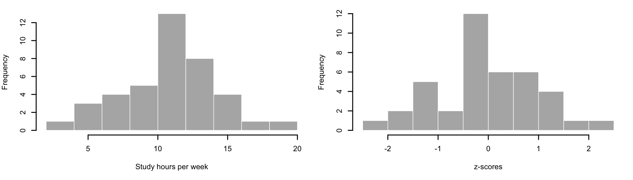
Rescaling changes only the numbers on the axis. As Figure 9.1 shows, the histogram of the z-scores has exactly the same shape as the histogram of the hours: the transformation does not make the data any more, or any less, normal77 For the same reason, the correlation between the two variables does not change: it is 0.56 for the raw values and 0.56 for the z-scores..
7 For the same reason, the correlation between the two variables does not change: it is 0.56 for the raw values and 0.56 for the z-scores.
9.1.2 An Example: Mean Centering
In Simple Linear Regression we predicted the exam scores of the same students from their study time. The intercept of that model, 44.34 points, is the predicted score of a student who does not study at all. Because none of the students studied less than 3.3 hours a week, the intercept was needed to position the line, but it did not describe an actual student. Mean centering the predictor solves this problem. Let’s subtract the mean study time, 10.70 hours, from each student’s hours and fit the model again.
Call:
lm(formula = exam ~ hours, data = cs)

Coefficients:
(Intercept)        hours
     44.341        2.222
Call:
lm(formula = exam ~ hours_c, data = cs)

Coefficients:
(Intercept)      hours_c
     68.125        2.222
The slope is the same in both models, 2.22 points per hour, because centering does not change the spread of the predictor. Only the intercept changes. In the centered model, a value of 0 for the predictor means “an average amount of study”, so the intercept, 68.12 points, is the predicted score of a student who studies an average number of hours88 In a simple linear regression, the intercept of the centered model is always equal to the mean of the criterion, because the line passes through the point defined by the two means.. Centering makes the intercept meaningful without changing anything else in the model. It becomes even more useful in Multiple Linear Regression, especially when the model includes interactions between predictors.
8 In a simple linear regression, the intercept of the centered model is always equal to the mean of the criterion, because the line passes through the point defined by the two means.
9.2 Distribution Normalization
There are many real world processes that generate data that do not follow the normal, Gaussian, distribution. Assumptions and Outliers already discussed how to determine if the data are normally distributed or not. Non-normal data usually fits in one of two categories: 1) follows a different distribution or 2) is a mixture of distributions and data generation processes.
For the data that follows a known distribution99 E.g., binomial, log-normal, exponential, etc., one can either identify the theoretical distribution it follows and analyze the data using tests appropriate for that distribution or somehow transform it to a normal distribution before analysis and then use tests that assume data distribution to be normal.
9 E.g., binomial, log-normal, exponential, etc.
Dealing with the 2nd category of non-normal data, which displays a mixture of distributions, is more complicated because few, if any, transformations would be able to deal with all that variability for the entire data set. In this case, the data needs to be studied and refined before analysis. For example, an attempt to break down the data can produce sub-samples or categories for which, individually, the distributions are known or recognizable. In this case, transformations can be applied to each sub-sample or category. If the observed data is produced by multiple processes, such as business data produced by complex work activities, multiple shifts, locations, customers, seasonality, etc., an attempt to review the individual process that produced data points and find a common denominator to transform the data to can sometimes help bring the data close enough to the normal distribution so that analysis is possible1010 The process always works better for larger samples.. An example is discussed in When a Transformation Cannot Help.
10 The process always works better for larger samples.
Some of the common options are:
- Box-Cox transformation: Uses a family of power functions, x^\lambda, to transform data to a more normal distribution form (Box and Cox 1964). The power \lambda is chosen from the data, as the value that brings the data closest to a normal distribution. The formula used for transformation are simple but computationally intensive, so the search is left to statistical software. Several of the transformations below are special cases: \lambda = 0.5 is the square root, and \lambda = 0 stands for the log.
- Log transformation: The value of each observation is transformed by applying the base 10 or natural logarithm to the observed value. The reverse process is to raise the values at the power of 10 or e1111 For the natural logarithms., depending of what type of logarithm was initially applied. It is especially useful if the original variable follows a log-normal distribution; after transformation the resulted values will be normally distributed. The logarithm is defined only for positive values, so it cannot be applied directly to data that includes zeros or negative values.
11 For the natural logarithms.
- Square-root transformation: The value of each observation is transformed by taking its square root. To reverse the process is to square the values. Usually used when the variable is a count of something. If the sample includes negative values, the sample should be first rescaled to have all positive values1212 For example by adding a certain amount to each observed value..
12 For example by adding a certain amount to each observed value.
- Arcsine transformation: The value of each observation is transformed by taking the arcsine of the square root of the number. The numbers to be transformed should be between 0 and 1. The resulted unit of measure is radians and the resulting range is 0 to \pi/2. It is usually useful for proportions or ratio type data that ranges between 0 and 11313 Its use has declined. For proportions computed from counts, such as the number of correct answers out of the number of questions, logistic regression is usually the better choice (Warton and Hui 2011). See Multiple Logistic Regression..
13 Its use has declined. For proportions computed from counts, such as the number of correct answers out of the number of questions, logistic regression is usually the better choice (Warton and Hui 2011). See Multiple Logistic Regression.
9.2.1 An Example: Log Transformation
The team that runs the course website redesigned its pages and wants to know whether the new version is easier to use. 70 participants were randomly assigned to complete the same task1414 Finding an assignment’s due date and submitting a file. on either the old or the new version of the website, 35 on each, and the time each of them took was recorded, in seconds. The data set1515 Column labels are: participant, group (old or new), time, and errors. was made up for this example.
14 Finding an assignment’s due date and submitting a file.
15 Column labels are: participant, group (old or new), time, and errors.
Completion times are a classic example of data that is not normally distributed. They cannot be shorter than zero, most people finish in a similar time, and a few take much longer. Let’s look at the data before choosing a test.
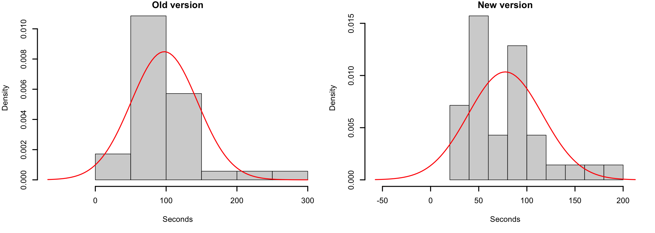
The histograms in Figure 9.2 show the typical shape of completion times: a peak on the left and a long tail to the right1616 The normal curve with the same mean and standard deviation even extends below zero, which completion times cannot do.. The Shapiro-Wilk test confirms the departure from normality for both the old version (p < .001) and the new version (p = .007). The assumption of normality of the independent samples t-Test is not met. Let’s take the natural logarithm of the times.
16 The normal curve with the same mean and standard deviation even extends below zero, which completion times cannot do.
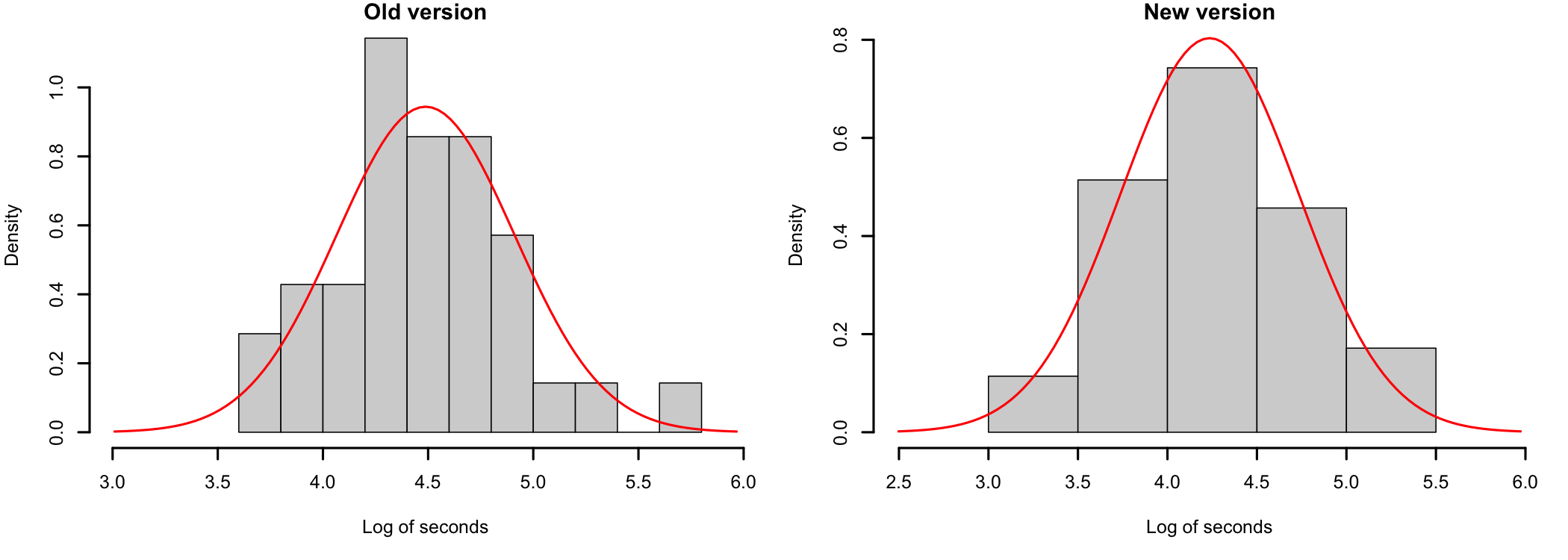
The log-transformed times (Figure 9.3) are much closer to the normal curve, and the Shapiro-Wilk test no longer indicates a departure from normality, for either the old version (p = .775) or the new version (p = .708). Much better. The analysis can now continue, on the log-transformed data.
Hypotheses.
- Null hypothesis (H0): In the population, the mean log completion time is the same for the two versions of the website (\mu_{new} = \mu_{old}, on the log scale).
- Alternative hypothesis (H1): In the population, the mean log completion times differ (\mu_{new} \neq \mu_{old}).
Decision criteria. The significance level is set at \alpha = .05, and the test is two-tailed. The test is the independent samples t-Test on the log-transformed times. H0 is rejected if the p-value is smaller than \alpha.
    Welch Two Sample t-test

data:  l.new and l.old
t = -2.2915, df = 66.303, p-value = 0.02512
alternative hypothesis: true difference in means is not equal to 0
95 percent confidence interval:
 -0.47261252 -0.03252878
sample estimates:
mean of x mean of y
 4.235494  4.488065
Decision. t(66.3) = -2.29, p = .025. The p-value is smaller than \alpha = .05. The null hypothesis is rejected: the completion times differ between the two versions of the website.
Effect size. On the log scale, Cohen’s d = 0.551717 See Effect Size and Power.. As discussed below, the difference is easier to understand once it is converted back to seconds.
17 See Effect Size and Power.
9.2.2 Converting the Results Back
Nobody thinks of time in “log seconds”, so the results have to be converted back to seconds. This is where log transformations are most often misreported. The reverse of the natural logarithm is the exponential function, e^x, and applying it to the results changes their meaning:
- The mean of the log values converts back to the geometric mean of the original values1818 The geometric mean of n values is the nth root of their product. For skewed data it is smaller than the arithmetic mean and closer to the median., not to their ordinary (arithmetic) mean. The geometric mean completion time was 88.9 seconds with the old version and 69.1 seconds with the new one. For comparison, the arithmetic means were 97.5 and 77.6 seconds, pulled up by the few participants who took much longer, and the medians were 89.1 and 65.3 seconds;
18 The geometric mean of n values is the nth root of their product. For skewed data it is smaller than the arithmetic mean and closer to the median.
- A difference between log values converts back to a ratio between the original values, because \log a - \log b = \log \frac{a}{b}. The difference between the means of the log times converts back to a ratio of 0.78, with a 95% confidence interval from 0.62 to 0.97.
In other words, a typical participant completed the task in about 22% less time with the new version of the website than with the old one (95% CI: 3% to 38%). A log transformation turns a question about differences into a question about ratios, which is often a more natural way to describe times, prices, or incomes.
Finally, here is an example of how to write up the results in a publication.
Completion times were positively skewed (Shapiro-Wilk p < .001 for the old version and p = .007 for the new version) and were log-transformed before the analysis. The log-transformed times did not depart significantly from normality (p = .775 and p = .708). An independent samples t-test on the log-transformed times showed that participants completed the task faster with the new version of the website (geometric mean = 69.1 s) than with the old version (geometric mean = 88.9 s), t(66.3) = -2.29, p = .025, d = 0.55. The ratio of the geometric means was 0.78, 95% CI [0.62, 0.97], a reduction of about 22% in completion time.
9.2.3 Square Root and Box-Cox
The participants in the study above also made a number of errors while completing the task. Counts like these have a property that complicates many tests: their variance grows with their mean. The participants who used the old version made 3.49 errors on average, with a variance of 4.49, while those who used the new version made 2.51 errors, with a variance of 2.26. The square root brings the variances closer together1919 After the transformation, the variances are 0.37 and 0.26. Their ratio drops from 1.99 to 1.42., which helps meet the assumption of homogeneity of variance2020 See Assumptions and Outliers..
19 After the transformation, the variances are 0.37 and 0.26. Their ratio drops from 1.99 to 1.42.
20 See Assumptions and Outliers.
Instead of guessing which transformation to use, the Box-Cox procedure can search for it. For the completion times, the best power is \lambda = 0.05, with a 95% confidence interval from -0.30 to 0.40. Because the interval includes 0, the log transformation used above is a good choice2121 In practice, a “round” value inside the confidence interval, such as 0 (log), 0.5 (square root), or 1 (no transformation), is preferred to the exact value, because it is much easier to interpret..
21 In practice, a “round” value inside the confidence interval, such as 0 (log), 0.5 (square root), or 1 (no transformation), is preferred to the exact value, because it is much easier to interpret.
9.2.4 When a Transformation Cannot Help
Transformations work when the data comes from a single process with a skewed distribution, such as the completion times above. They do not work when the data is a mixture. Consider the hours of paid work of the 40 students in the course. 13 of them (32%) do not work at all, and the others work from 1 to 43 hours a week. The data is not normally distributed (Shapiro-Wilk p < .001).
The log cannot be applied directly, because the logarithm of zero is not defined. A common workaround is to add 1 to every value before taking the log. It does not help here: the 13 zeros become 13 identical values at the bottom of the distribution, and the transformed data is still far from normal (p = .001)2222 No transformation can spread out 13 identical values. Whatever the formula, they stay identical..
22 No transformation can spread out 13 identical values. Whatever the formula, they stay identical.
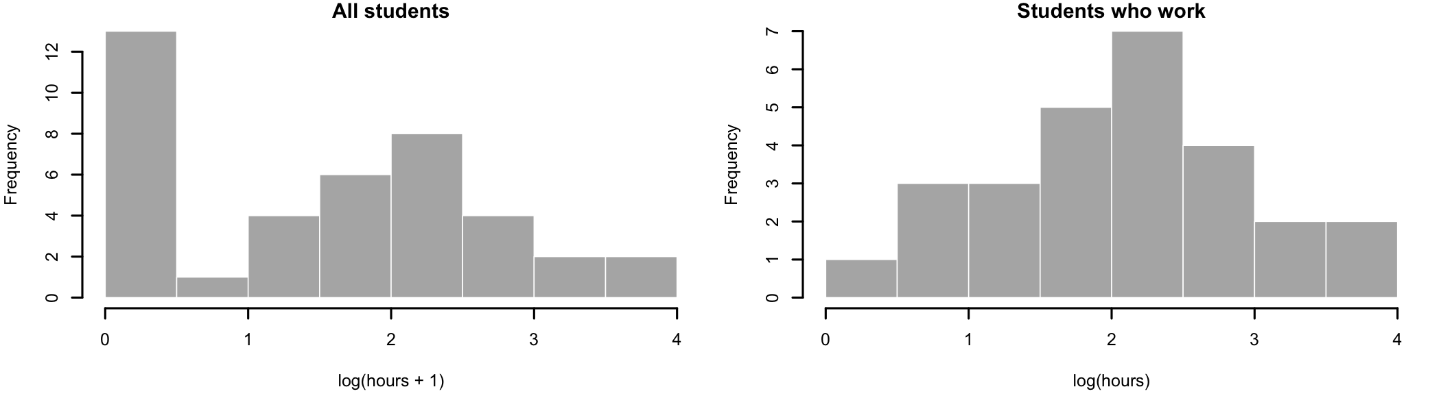
The data describes two different groups: the students who do not work, and those who do. As discussed earlier in this chapter, the better approach is to separate them. The question “Does the student work?” becomes a categorical variable, analyzed with the methods for categorical data, and the hours of the 27 students who work can be studied on their own. For them alone, the log transformation works well (Figure 9.4, right): the log-transformed hours do not depart from normality (p = .919).
9.3 Summary
Rescaling, such as min-max normalization, mean centering, and z-scores, changes the units of the data but not its shape. It is used to compare or combine variables measured on different scales, and to make the results of a model easier to interpret. It does not make data any more normal.
Transformations such as the log, the square root, or the Box-Cox family change the shape of the data, and can bring a skewed distribution close enough to normal for tests that assume normality. Of note is the fact that the results of a transformed analysis must be converted back, and that the converted results change meaning: the mean of log values becomes a geometric mean, and a difference becomes a ratio. Finally, no transformation can fix data that mixes different groups or processes. Such data has to be separated first.