11 Equivalence Testing
At a glance
- Question
- Are two groups the same, within a margin set in advance?
- Design
- Two independent groups, one measurement of each participant
- Dependent variable
- Interval or ratio
- Independent variable
- Nominal, two levels
- Assumptions
-
- The equivalence margin is set and justified before the data is collected
- Independent observations: each participant belongs to one group only
- DV normally distributed in each group (Welch’s version does not need equal variances)
- Null hypothesis
- The difference is at least as large as the margin (\theta \leq -\varepsilon or \theta \geq +\varepsilon)
- Test statistic
- Two one-sided t tests (TOST), one against each end of the margin
- Effect size
- The mean difference with its 90% CI, and Cohen’s d
- If conditions fail
-
- The DV is ordinal, or clearly not normal in a small sample → A rank-based equivalence test, with its margin set on the scale of what it compares
- Include in the write-up
-
- The margin, and why it was chosen
- The size, mean, and standard deviation of each group, and the normality checks
- Both one-sided tests: t(df) = …, p = …
- The 90% CI of the difference, and whether it lies inside the margin
Used to show that two groups are the same, within a margin set by the researcher, rather than different. Equivalence testing answers questions such as: Does a new, cheaper instrument measure the same thing as the established one? Does an online version of a study produce the same results as the laboratory version? Does a generic drug work as well as the original?11 Equivalence testing was first developed in the pharmaceutical industry, to show that a generic drug is absorbed by the body in the same way as the original (Schuirmann 1987; Wellek 2010).
1 Equivalence testing was first developed in the pharmaceutical industry, to show that a generic drug is absorbed by the body in the same way as the original (Schuirmann 1987; Wellek 2010).
Most of the tests in this book, such as the t-Test, are built to detect differences. Their null hypothesis states that there is no difference, and a significant result is evidence that there is one. A non-significant result, however, is not evidence that the groups are the same. It only means that the data did not provide enough evidence of a difference, which may be because there is no difference, or because the sample was too small, or the measurements too noisy, to detect it22 Hence the saying: “absence of evidence is not evidence of absence”.. To claim that two groups are the same, the hypotheses have to be reversed. This is what equivalence testing does.
2 Hence the saying: “absence of evidence is not evidence of absence”.
11.1 The Theory
11.1.1 Reversing the Hypotheses
No two groups are ever exactly the same, so equivalence is always defined with respect to a margin33 Also called the equivalence bound, equivalence interval, or tolerance, and usually written \varepsilon or \Delta. \varepsilon: the largest difference that is still too small to matter. If \theta is the difference between the two population means, the hypotheses are:
3 Also called the equivalence bound, equivalence interval, or tolerance, and usually written \varepsilon or \Delta.
- Null hypothesis (H0): The difference is at least as large as the margin, \theta \leq -\varepsilon or \theta \geq +\varepsilon. The groups are not equivalent;
- Alternative hypothesis (H1): The difference is smaller than the margin, -\varepsilon < \theta < +\varepsilon. The groups are equivalent.
Of note is the fact that the burden of proof is now on equivalence. If the data is too noisy or the sample too small, the test fails to reject H0 and the groups cannot be declared equivalent. A study that is too small to detect a difference is also too small to show equivalence.
11.1.2 The Equivalence Margin
The margin is the most important decision in an equivalence test, and it must be made before the data is collected44 Choosing the margin after seeing the data makes it possible to pick the one that gives the desired result.. It is the smallest effect size of interest: any difference smaller than the margin is considered too small to matter in practice (Lakens et al. 2018). There is no single rule for setting it. The common approaches are:
4 Choosing the margin after seeing the data makes it possible to pick the one that gives the desired result.
- Raw units, based on what is practically meaningful. For example, a difference of less than 2 points on a 100-point test may be of no consequence for a placement decision;
- Standardized units, a fraction of the standard deviation, such as \varepsilon = 0.5 \times SD, which corresponds to a medium effect size55 See Effect Size and Power.. The standard deviation has to come from prior research or a pilot study, not from the data being tested;
5 See Effect Size and Power.
- Field conventions, when a discipline has agreed on a margin66 In pharmacology, for example, two drugs are considered bioequivalent when the ratio of their average absorption falls between 80% and 125%. Communication research has used margins of 20% of the scale or of the control group’s mean (Weber and Popova 2012)..
6 In pharmacology, for example, two drugs are considered bioequivalent when the ratio of their average absorption falls between 80% and 125%. Communication research has used margins of 20% of the scale or of the control group’s mean (Weber and Popova 2012).
11.1.3 Two One-Sided Tests
The most common procedure, called TOST (two one-sided tests) (Schuirmann 1987), splits the null hypothesis into its two parts and tests each one with a one-sided t-Test:
- The lower test checks whether the difference is larger than the lower bound, -\varepsilon: t_{L} = \frac{(\bar{X}_1 - \bar{X}_2) - (-\varepsilon)}{SE}
- The upper test checks whether the difference is smaller than the upper bound, +\varepsilon: t_{U} = \frac{(\bar{X}_1 - \bar{X}_2) - \varepsilon}{SE}
In both equations SE is the standard error of the difference between the means, the same one used by the independent samples t-Test. Equivalence is declared only if both tests are significant. The p-value of the TOST procedure is therefore the larger of the two p-values.
The same decision can be made with a confidence interval. The two groups are equivalent at \alpha = .05 if the 90% confidence interval of the difference lies entirely between -\varepsilon and +\varepsilon77 A 90% interval, and not 95%, because each of the two one-sided tests uses \alpha = .05 at one end of the interval. The interval leaves out 5% at each end, which is a confidence level of 1 - 2\alpha..
7 A 90% interval, and not 95%, because each of the two one-sided tests uses \alpha = .05 at one end of the interval. The interval leaves out 5% at each end, which is a confidence level of 1 - 2\alpha.
11.1.4 Difference and Equivalence Together
A test of difference and a test of equivalence answer different questions, and they can be run on the same data. At \alpha = .05, the test of difference rejects its null hypothesis when the 95% confidence interval excludes zero, and the test of equivalence when the 90% interval lies inside the margin. Together, they lead to one of four conclusions, shown in Figure 11.188 For simplicity, the figure shows one interval for each case, as if the 90% and the 95% intervals led to the same decision. In real data, check each decision with its own interval.:
8 For simplicity, the figure shows one interval for each case, as if the 90% and the 95% intervals led to the same decision. In real data, check each decision with its own interval.
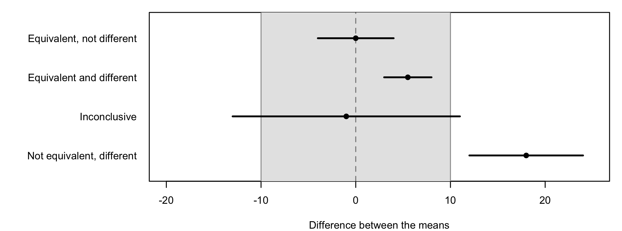
- Equivalent, not different: the interval lies inside the margin and includes zero. The best support for the claim that the groups are the same;
- Equivalent and different: the interval lies inside the margin, but does not include zero. The difference is real, but too small to matter99 With very large samples, even tiny differences become statistically significant. Equivalence testing helps judge whether they matter.;
9 With very large samples, even tiny differences become statistically significant. Equivalence testing helps judge whether they matter.
- Inconclusive: the interval includes zero, but extends beyond the margin. Neither a difference nor equivalence is shown, usually because the sample is too small. A failed equivalence test does not show that the groups differ;
- Not equivalent, different: the interval lies entirely outside the margin. The groups are different, by more than the margin.
11.2 Assumptions
Because each of the two one-sided tests is a t-Test, the TOST procedure for two independent groups has the same assumptions as the independent samples t-Test:
- Independence of observations
- Usually ensured by the design of the study1010 E.g., each participant is randomly assigned to one group only and is measured once.;
10 E.g., each participant is randomly assigned to one group only and is measured once.
- Violated when participants belong to both groups, or influence each other’s responses.
- Usually ensured by the design of the study1010 E.g., each participant is randomly assigned to one group only and is measured once.;
- Normal distribution of the data in each group
- Detected using normal probability (q-q) plots and tests of normality;
- Violated when the points fall far from the straight line of the plot. When normality cannot be assumed in a small sample, rank-based equivalence tests exist (Wellek 2010), but they test the equivalence of a different quantity, such as how often a score in one group is higher than a score in the other, so their margin has to be set on that scale.
The version of the t-Test used here, Welch’s t-Test, does not require the two groups to have equal variances1111 See the independent samples t-Test..
11 See the independent samples t-Test.
11.3 The Study
Researchers who study how people react to political debates, commercials, or comedy often use real-time response measurement: while watching a video, participants move a slider to show, second by second, how much they like what they see. Traditionally, this requires a laboratory with dedicated hardware. A research team wants to know whether an on-screen slider, used in a web browser on the participants’ own devices, can replace the hardware slider1212 The study is modeled on the design of a published study comparing hardware and on-screen sliders (Ionas and Geana 2026), simplified for this chapter.. The question asked is: Does the on-screen slider produce the same responses as the hardware slider?
12 The study is modeled on the design of a published study comparing hardware and on-screen sliders (Ionas and Geana 2026), simplified for this chapter.
100 participants were randomly assigned to one of two groups. The 50 participants in the first group watched a 60-second comedy clip in the laboratory and used a hardware slider. The 50 participants in the second group watched the same clip at home and used an on-screen slider in their browser. Both sliders ranged from 0 (not funny at all) to 100 (very funny)1313 The two devices record the slider’s position at different rates, and the browser’s rate varies with the device. Before any comparison, the raw recordings were averaged to one value per second and aligned with the timeline of the clip. The data set used here starts after these steps.. The data set1414 Column labels are: participant, group (hardware or virtual), second, and value. was made up for this example. The first few rows are shown in Table 11.1.
13 The two devices record the slider’s position at different rates, and the browser’s rate varies with the device. Before any comparison, the raw recordings were averaged to one value per second and aligned with the timeline of the clip. The data set used here starts after these steps.
14 Column labels are: participant, group (hardware or virtual), second, and value.
| Participant | Group | Second | Value |
|---|---|---|---|
| 1 | hardware | 1 | 8.1 |
| 1 | hardware | 2 | 7.9 |
| 1 | hardware | 3 | 1.7 |
| 1 | hardware | 4 | 11.8 |
| 1 | hardware | 5 | 11.9 |
| 1 | hardware | 6 | 21.4 |
The analysis is done in two steps. First, we compare the two sliders on the average response of each participant over the whole clip. Then, as in the published study, we compare them second by second.
11.4 The Whole Clip
For each participant, the 60 values were averaged into one score, the participant’s mean response to the clip.
Hypotheses. Let \theta be the difference between the mean responses of the hardware and the on-screen slider in the population, \theta = \mu_{hardware} - \mu_{virtual}.
- Null hypothesis (H0): The two sliders are not equivalent, \theta \leq -10 or \theta \geq 10.
- Alternative hypothesis (H1): The two sliders are equivalent, -10 < \theta < 10.
Decision criteria. The margin was set before the data was collected. In a pilot study, the standard deviation of the participants’ mean responses was about 20 points, so a medium effect of half a standard deviation gives \varepsilon = 10 points1515 Ten points is also 10% of the range of the scale, a stricter margin than the 20% used in some communication research.. The significance level is \alpha = .05 for each of the two one-sided tests, which corresponds to a 90% confidence interval. H0 is rejected, and the sliders declared equivalent, if both p-values are smaller than \alpha. The effect size is Cohen’s d.
15 Ten points is also 10% of the range of the scale, a stricter margin than the 20% used in some communication research.
11.4.1 Checking the Assumptions
The independence of observations is ensured by the design: each participant was assigned to one group only and watched the clip on their own.
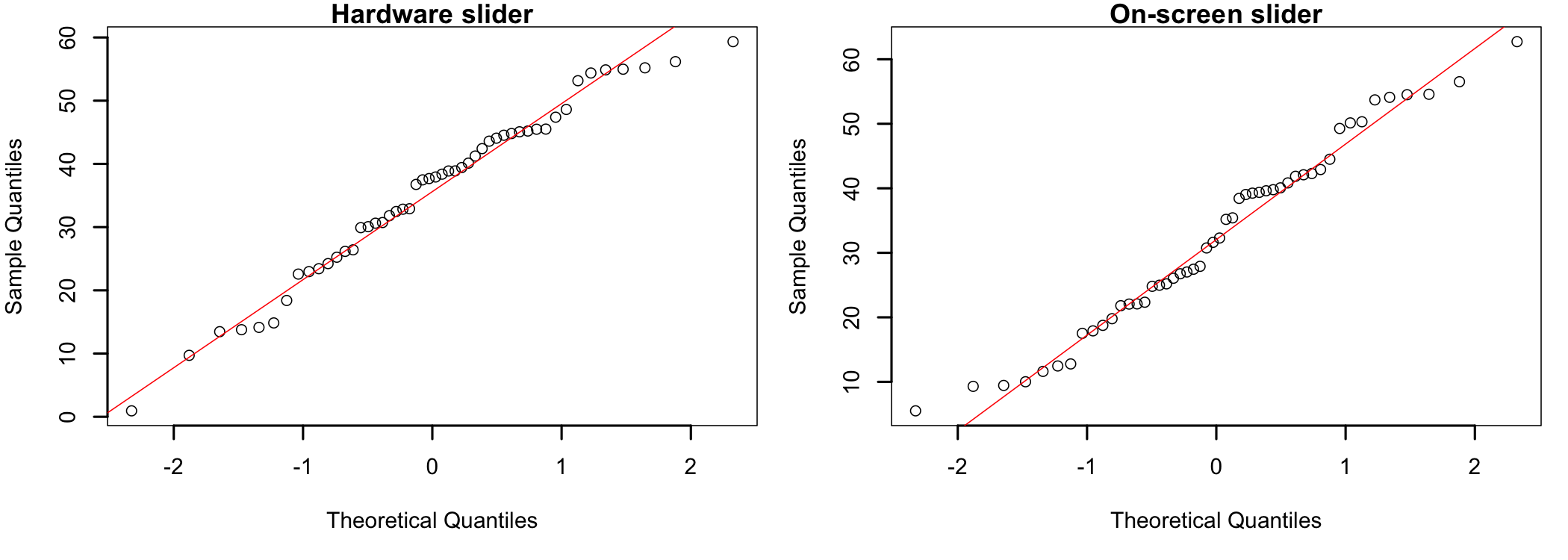
The points of both q-q plots (Figure 11.2) are close to the straight line, and the Shapiro-Wilk tests do not indicate a departure from normality for either the hardware slider (p = .323) or the on-screen slider (p = .307). The assumptions are met.
11.4.2 The Test
Let’s first look at the two groups and then run the usual test of difference, an independent samples t-Test.
$hardware
       n        M       SD
50.00000 35.58390 13.54196

$virtual
      n       M      SD
50.0000 32.4950 14.5058
    Welch Two Sample t-test

data:  x.hw and x.vs
t = 1.1007, df = 97.54, p-value = 0.2738
alternative hypothesis: true difference in means is not equal to 0
95 percent confidence interval:
 -2.480699  8.658499
sample estimates:
mean of x mean of y
  35.5839   32.4950
The participants who used the hardware slider gave a mean response of 35.58 (SD = 13.54), and those who used the on-screen slider 32.49 (SD = 14.51). The difference of 3.09 points is not significant, t(97.5) = 1.10, p = .274. As discussed above, this does not mean that the two sliders are the same. Let’s run the two one-sided tests.
    Welch Two Sample t-test

data:  x.hw and x.vs
t = 4.6639, df = 97.54, p-value = 4.933e-06
alternative hypothesis: true difference in means is greater than -10
95 percent confidence interval:
 -1.571532       Inf
sample estimates:
mean of x mean of y
  35.5839   32.4950
    Welch Two Sample t-test

data:  x.hw and x.vs
t = -2.4626, df = 97.54, p-value = 0.007774
alternative hypothesis: true difference in means is less than 10
95 percent confidence interval:
     -Inf 7.749332
sample estimates:
mean of x mean of y
35.5839 32.4950 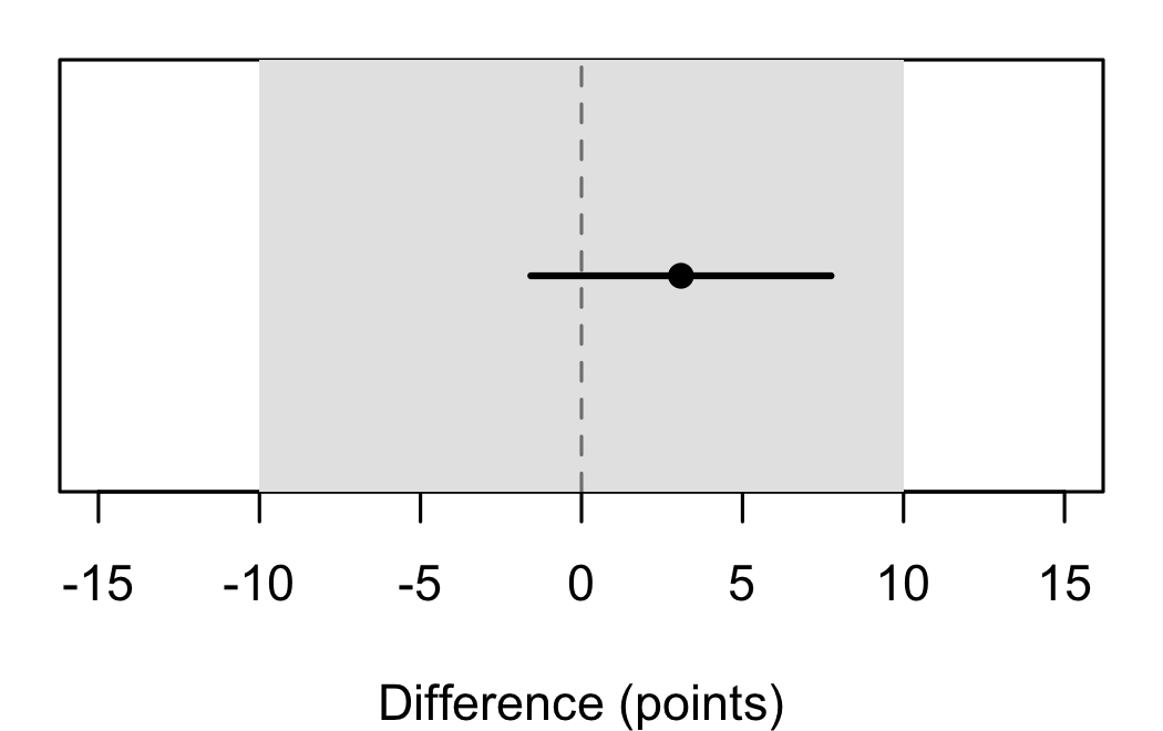
Decision. The lower test shows that the difference is larger than -10, t(97.5) = 4.66, p < .001, and the upper test shows that it is smaller than 10, t(97.5) = -2.46, p = .008. Both p-values are smaller than \alpha = .05. The null hypothesis is rejected and the alternative hypothesis accepted: the two sliders are equivalent within ±10 points. The same conclusion follows from the 90% confidence interval of the difference, -1.57 to 7.75, which lies entirely inside the margin (Figure 11.3). Together with the non-significant t-Test, the result falls in the first of the four cases of Figure 11.1: equivalent, and not different.
Effect size. The difference between the two sliders is 3.09 points, d = 0.22, a small effect1616 Cohen’s d is the difference between the means divided by the pooled standard deviation. See Effect Size and Power..
16 Cohen’s d is the difference between the means divided by the pooled standard deviation. See Effect Size and Power.
Of note is the fact that the conclusion depends on the margin. With a stricter margin of ±5 points, the same data would not show equivalence: the upper end of the confidence interval (7.75) is above 5, and the upper test is not significant (p = .249). This is why the margin has to be chosen, and justified, before the analysis.
11.5 Second by Second
Real-time response data is used to find the moments of a video that people react to, so it matters whether the two sliders agree at every moment, and not only on average. The published study answered this question by repeating the equivalence test for each second of the video1717 Each second is compared on its own, as a separate snapshot. The snapshots are not independent of each other, since the same participants respond at every second, so they describe where the sliders agree rather than adding up to a test of the whole clip. This is not a time series analysis, which would model how the responses change from one second to the next.. The result is the percentage of seconds for which the two sliders are equivalent.
17 Each second is compared on its own, as a separate snapshot. The snapshots are not independent of each other, since the same participants respond at every second, so they describe where the sliders agree rather than adding up to a test of the whole clip. This is not a time series analysis, which would model how the responses change from one second to the next.
With the same margin of ±10 points, the two sliders are equivalent for 43 of the 60 seconds (72%). Figure 11.4 shows where the other seconds are.
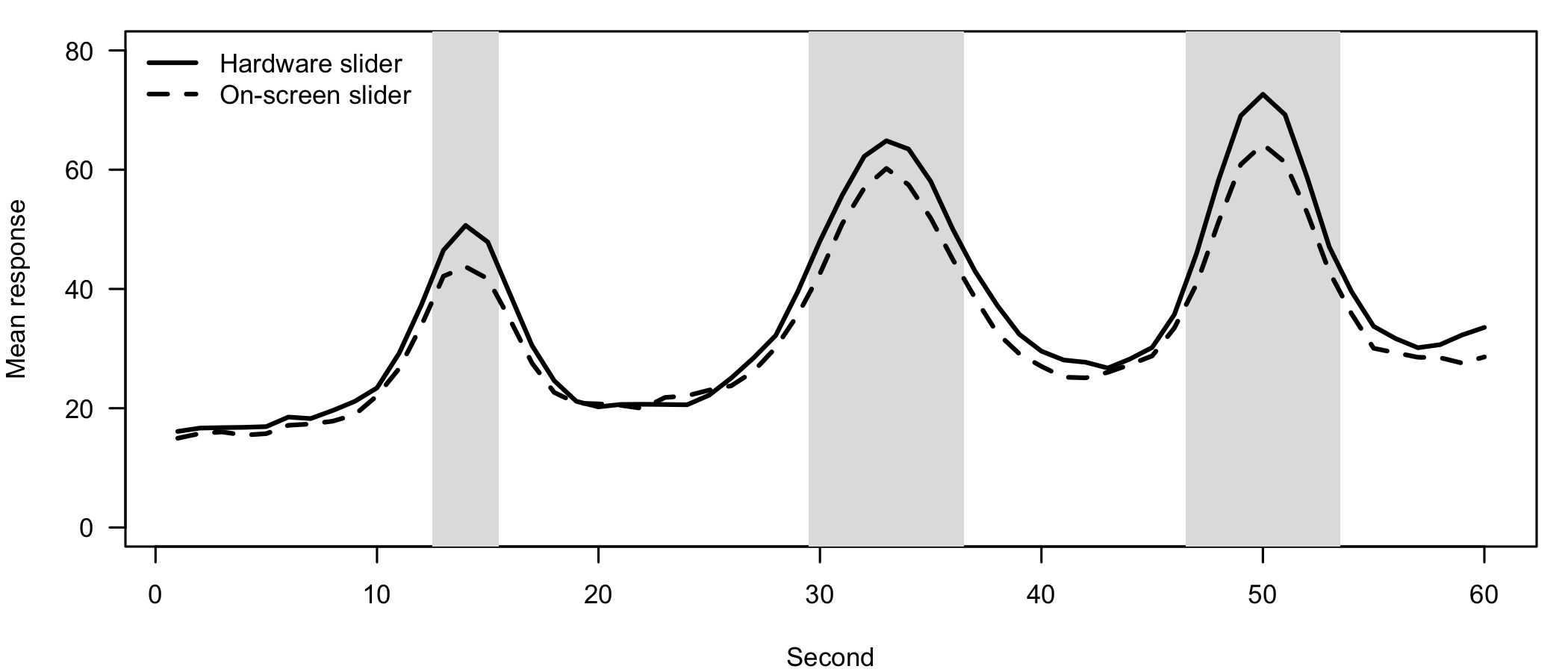
The two curves rise and fall together: both sliders capture the same three jokes at the same moments. The seconds for which equivalence is not shown cluster around the peaks of the jokes, where the on-screen slider stays a few points below the hardware slider. The same pattern was observed in the published study (Ionas and Geana 2026). Two reasons combine here. The difference between the sliders is largest at the peaks, and so is the spread of the responses1818 The standard deviation of the responses ranges from 10.6 points at the quietest second to 25.1 points at the peaks., which widens the confidence interval of the difference.
18 The standard deviation of the responses ranges from 10.6 points at the quietest second to 25.1 points at the peaks.
Of note is the fact that the second-by-second results are more demanding than the whole-clip result. A participant’s mean over 60 seconds varies much less than their response at a single second, so the same margin is easier to meet on average than at each moment.
11.5.1 How Sensitive Is the Result to the Margin?
A single margin hides how close the decision was. The published study also reported a sensitivity curve: the percentage of equivalent seconds for every margin from 1 to 25 points.
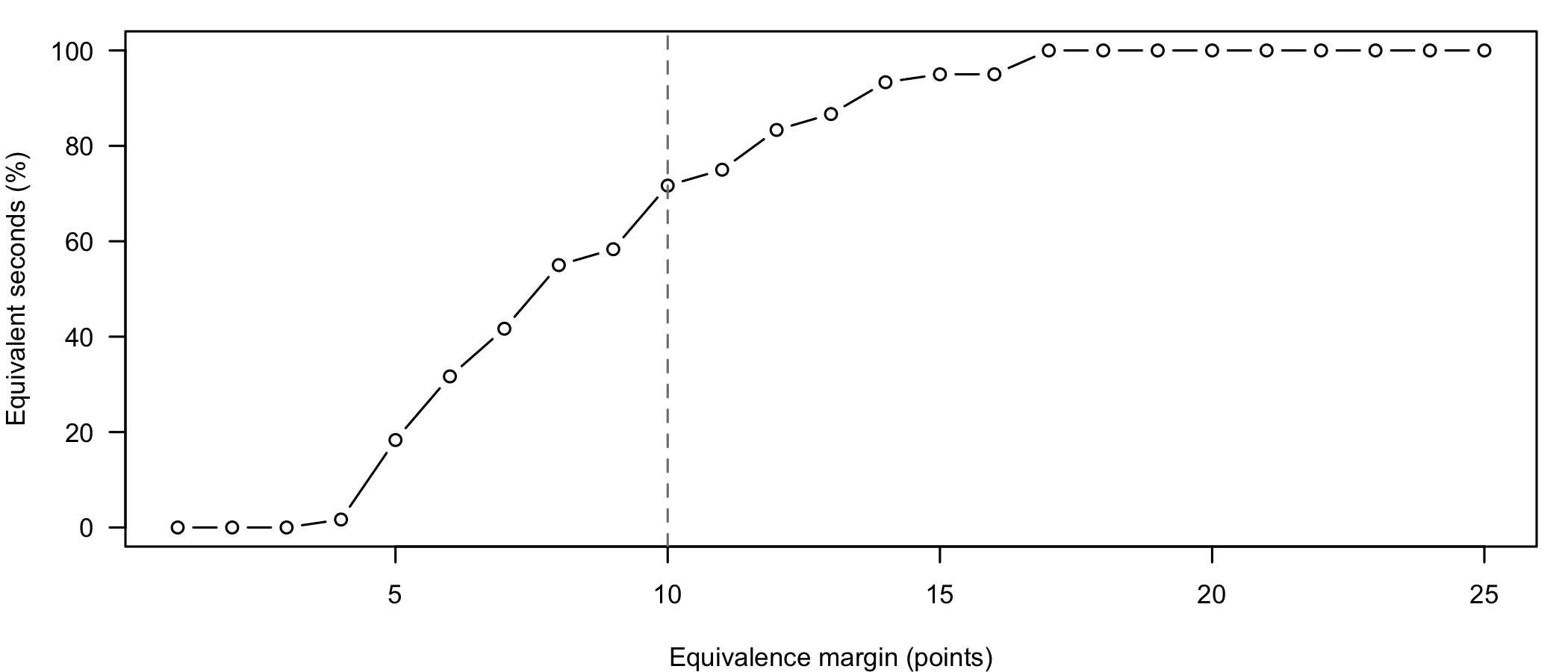
The curve (Figure 11.5) shows that no second is equivalent at very small margins. The percentage rises quickly between 5 and 15 points, reaches 80% at a margin of 12 points, and 100% at 17 points. A reader who prefers a stricter or a more lenient margin than ours can read the result for that margin directly from the curve1919 The published study used a margin of 20% of the scale, and reported that 80% of the seconds were equivalent at margins well below it (Ionas and Geana 2026)..
19 The published study used a margin of 20% of the scale, and reported that 80% of the seconds were equivalent at margins well below it (Ionas and Geana 2026).
Two cautions apply to the second-by-second analysis. First, the percentage of equivalent seconds is a description, not a test. Consecutive seconds are not independent of each other, and how high the percentage has to be is a judgment the researcher must make and justify, just like the margin. Second, with 60 tests, a few of them are expected to reach the wrong decision by chance alone2020 See The p-Value Controversy.. Isolated non-equivalent seconds deserve less attention than the clusters, such as those around the peaks of the jokes.
20 See The p-Value Controversy.
11.5.2 Reporting the Results
Finally, here is an example of how to write up the results in a publication.
Equivalence between the hardware and the on-screen slider was tested with the two one-sided tests (TOST) procedure, using equivalence bounds of ±10 points (half the standard deviation observed in a pilot study). The participants’ mean responses to the clip did not depart significantly from normality (Shapiro-Wilk p = .323 for the hardware slider and p = .307 for the on-screen slider). The mean response of the participants who used the hardware slider (M = 35.58, SD = 13.54, n = 50) was not significantly different from that of the participants who used the on-screen slider (M = 32.49, SD = 14.51, n = 50), t(97.5) = 1.10, p = .274, d = 0.22. Both one-sided tests were significant, t(97.5) = 4.66, p < .001 for the lower bound and t(97.5) = -2.46, p = .008 for the upper bound, 90% CI [-1.57, 7.75], and the two sliders were considered equivalent. Tested second by second with the same bounds, the sliders were equivalent for 43 of the 60 seconds (72%). The seconds for which equivalence was not shown clustered around the peaks of the responses, where the on-screen slider recorded lower values.
11.6 Summary
Equivalence testing reverses the usual hypotheses: the null hypothesis states that the groups differ by at least a set margin, and rejecting it supports the claim that they are the same. The TOST procedure does this with two one-sided t-Tests, one for each bound of the margin, and equivalence is declared only when both are significant, or, equivalently, when the 90% confidence interval of the difference lies inside the margin.
In our example, the on-screen slider produced the same mean responses to the clip as the hardware slider, within ±10 points. Second by second, the two sliders followed the same pattern, but equivalence was not shown at the moments of strongest reaction, where the on-screen slider recorded lower values. Of note is the fact that the margin decides the answer. It must be set before the data is collected, justified by prior research, practical considerations, or field conventions, and reported together with the results.