13 Factorial ANOVA and Interactions
At a glance
- Question
- Do two factors affect the mean of a DV, and does the effect of one depend on the other?
- Design
- Two or more independent variables, crossed, with different participants in each cell
- Dependent variable
- Interval or ratio
- Independent variables
- Two or more factors, nominal, each with two or more levels
- Assumptions
-
- Independent observations: each participant is in one cell only
- DV normally distributed in each cell
- Equal variances in the cells (Levene’s test)
- Null hypothesis
- Three null hypotheses: no main effect of each factor, and no interaction
- Test statistic
- F for each main effect and for the interaction
- Effect size
- Partial \eta^{2} (\eta^{2}_{p}): .01 small, .06 medium, .14 large
- If conditions fail
-
- The interaction is significant → Simple effects: the effect of one factor at each level of the other
- A factor is a repeated measurement of the same participants → Mixed designs
- Include in the write-up
-
- The design (for example 2 \times 3), and the cell means and standard deviations
- The assumption checks for the cells
- F(df1, df2) = …, p = …, and \eta^{2}_{p} for each effect
- The simple effects when the interaction is significant
Used to study the effects of two or more independent (predictor) variables, called factors, on one dependent (criterion) variable measured on an interval or ratio scale. Each factor has two or more levels, and the design includes every combination of the levels of the factors, called cells11 A study that crosses two methods of instruction with three class sizes, for example, has 2 \times 3 = 6 cells.. The analysis is called a two-way ANOVA, after the number of factors22 With three factors, a three-way ANOVA, and so on. The name factorial ANOVA covers all of them..
1 A study that crosses two methods of instruction with three class sizes, for example, has 2 \times 3 = 6 cells.
2 With three factors, a three-way ANOVA, and so on. The name factorial ANOVA covers all of them.
Compared with a separate one-way ANOVA for each factor, the factorial design has three advantages:
- Economy, because the same participants provide information about all factors at once;
- Precision, because the variability explained by the second factor is removed from the error term, which makes the tests of both factors more powerful;
- Interactions, because it shows whether the effect of one factor depends on the level of the other. This is the reason most factorial designs are used.
The second part of the chapter extends the idea of interaction to predictors measured on a continuous scale, using regression.
13.1 Main Effects and Interactions
A main effect is the effect of one factor on the dependent variable, averaged across the levels of the other factor. An interaction exists when the effect of one factor is not the same at all levels of the other factor33 When the theory states that a third variable changes the strength or the direction of the relationship between an independent and a dependent variable, the interaction is called moderation. The statistical analysis is the same. See Moderating vs. Mediating Variables.. For example, a medication may lower blood pressure in younger patients and have no effect in older ones. In this case, the effect of the medication depends on age.
3 When the theory states that a third variable changes the strength or the direction of the relationship between an independent and a dependent variable, the interaction is called moderation. The statistical analysis is the same. See Moderating vs. Mediating Variables.
The easiest way to understand main effects and interactions is to look at a plot of the cell means, called an interaction plot. Figure 13.1 shows four possible results of a 2 \times 2 design, with factor A on the horizontal axis and the two levels of factor B as separate lines.
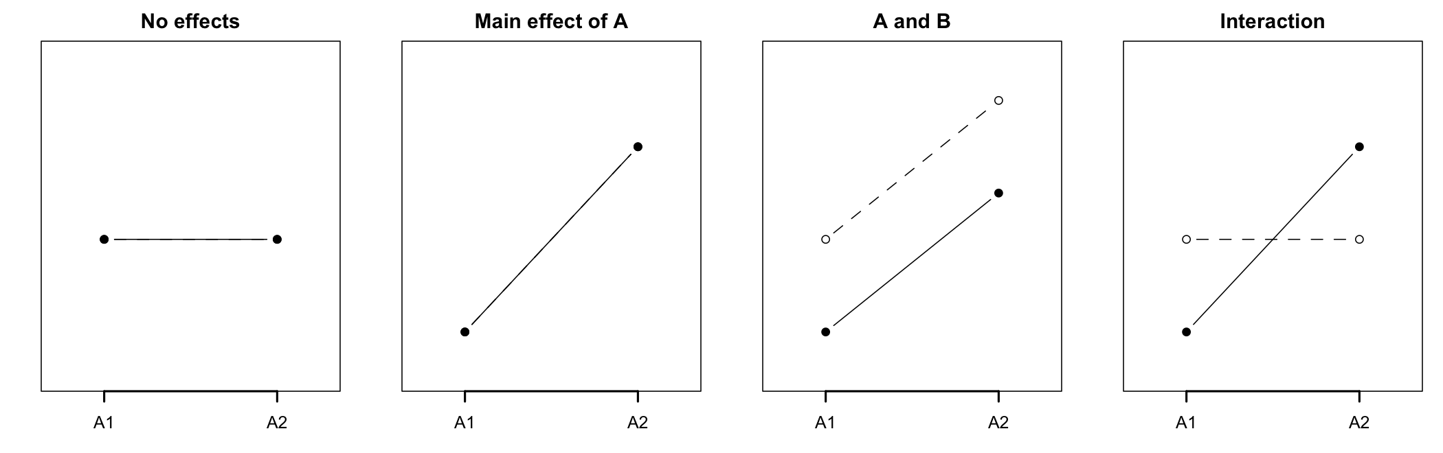
- When the lines are flat and on top of each other, neither factor has an effect;
- When the lines rise or fall, factor A has an effect. When the lines are separated, factor B has an effect;
- When the lines are not parallel, there is an interaction. In the last panel, A has a strong effect for one level of B and none for the other.
Of note is the fact that when an interaction is present, the main effects can be misleading. In the last panel of Figure 13.1, averaging across the levels of B shows an effect of A, but the effect exists only for one level of B. For this reason, the interaction is always interpreted first.
13.2 The Theory
13.2.1 Partitioning the Variance
The total variability is split as in the one-way ANOVA, into a model and a residual part. The model part is then split again, into one part for each main effect and one for the interaction. For two factors, A and B:
SS_{T} = SS_{A} + SS_{B} + SS_{A \times B} + SS_{R}
The residual sum of squares is computed from the distance of each score to the mean of its own cell. Each sum of squares is divided by its degrees of freedom to compute a mean square, and each effect is tested with an F ratio that uses the same error term, MS_{R}. With a levels of factor A, b levels of factor B, and N participants (Table 13.1):
| Source | Degrees of freedom | F |
|---|---|---|
| A | $a - 1$ | $MS_{A} / MS_{R}$ |
| B | $b - 1$ | $MS_{B} / MS_{R}$ |
| A × B | $(a - 1)(b - 1)$ | $MS_{A \times B} / MS_{R}$ |
| Residual | $N - ab$ | |
| Total | $N - 1$ |
The factorial ANOVA requires a fully crossed design: every level of one factor is combined with every level of the other. When some combinations are missing, or when the levels of one factor exist only within the levels of another44 For example, classes within schools: each class belongs to only one school. Such designs are called nested and are analyzed with multilevel models., the analysis is different.
4 For example, classes within schools: each class belongs to only one school. Such designs are called nested and are analyzed with multilevel models.
13.2.2 Types of Sums of Squares
When all cells have the same number of participants, the design is balanced, and the factors are independent of each other. When the cells have different sizes, the factors are correlated, and part of the variability can be attributed to either of them. There are three ways, called types, of dividing this shared part:
- Type I (sequential) sums of squares give the shared part to the factor entered first in the model. The results depend on the order of the factors;
- Type II sums of squares test each main effect after the other main effect, but ignore the interaction. They are appropriate when there is no interaction;
- Type III sums of squares test each effect after all the others, including the interaction. They do not depend on the order of the factors and are the most common choice in the social sciences.
In a balanced design, all three types give the same results.55 With unbalanced designs, Type III sums of squares require the factors to be coded with sum-to-zero (effect) codes, which compare each level with the grand mean, instead of the usual dummy codes.
5 With unbalanced designs, Type III sums of squares require the factors to be coded with sum-to-zero (effect) codes, which compare each level with the grand mean, instead of the usual dummy codes.
13.2.3 Effect Size
In a factorial design, the effect size of each effect is usually the partial eta squared (\eta^{2}_{p}), the variability explained by the effect, relative to that variability plus the error:
\eta^{2}_{p} = \frac{SS_{effect}}{SS_{effect} + SS_{R}}
Unlike \eta^{2}, the partial eta squared of an effect is not reduced by the variability explained by the other factors, which makes it comparable with the effect of the same factor in a one-way design66 For the same reason, the partial eta squared values of a design can add up to more than 1.. They are read with the same guidelines as \eta^{2}: .01 small, .06 medium, and .14 or more large.
6 For the same reason, the partial eta squared values of a design can add up to more than 1.
13.3 Assumptions
The assumptions are those of the one-way ANOVA, applied to the cells of the design:
- Independence of observations
- Usually ensured by the design of the study, with each participant in only one cell;
- Violated when the participants influence each other or are measured more than once. A factor whose levels are measurements of the same participants makes the study a mixed design, with its own analysis.
- The dependent variable (DV) is normally distributed in each cell
- Detected using q-q plots and tests of normality for each cell, or for the residuals of the model;
- Violated when the distributions are strongly skewed or have outliers.
- Homogeneity of variances across the cells
- Detected using Levene’s test on the cells of the design;
- Violated when the variances differ, which is more serious when the cells also differ in size.
13.4 The Study
A language instructor wanted to know how students should practice new vocabulary. Sixty students learned the same 40 words in a foreign language. They were randomly assigned to one of three practice methods: reading the list of words and their translations again (Rereading), writing a short summary that used the words (Summaries), or testing themselves with flash cards (Self-testing). Within each method, half of the students practiced in one long session (Massed) and the other half in three short sessions spread over a week (Spaced), for the same total time. A week after the last session, all students were asked to translate the 40 words. The design is a 2 (schedule) \times 3 (method) between-subjects factorial, with 10 students in each cell. The data set77 Column labels are: student, schedule, method, and recall, the number of words translated correctly. was made up for this example. The first few rows of the data set are shown in Table 13.2.
7 Column labels are: student, schedule, method, and recall, the number of words translated correctly.
| Student | Schedule | Method | Words recalled |
|---|---|---|---|
| 1 | Massed | Rereading | 9 |
| 2 | Massed | Rereading | 12 |
| 3 | Massed | Rereading | 12 |
| 4 | Massed | Rereading | 15 |
| 5 | Massed | Rereading | 11 |
| 6 | Massed | Rereading | 13 |
Hypotheses. A two-way ANOVA tests three pairs of hypotheses, one for each effect:
- Main effect of schedule. H0: In the population, the mean recall is the same for massed and spaced practice. H1: The mean recall differs between the two schedules.
- Main effect of method. H0: In the population, the mean recall is the same for the three practice methods. H1: At least one method differs from the others.
- Interaction. H0: The effect of the schedule is the same for all three methods. H1: The effect of the schedule depends on the method.
Decision criteria. The significance level is set at \alpha = .05 for each effect. With 60 students in 6 cells, the error term has 60 - 6 = 54 degrees of freedom. H0 is rejected for an effect if its p-value is smaller than \alpha. The effect size is \eta^{2}_{p}. If the interaction is significant, it is followed up with simple effects before the main effects are interpreted.
13.4.1 Describing the Cells
| Massed | Spaced | |
|---|---|---|
| Rereading | 12.50 (2.64) | 15.20 (3.99) |
| Summaries | 16.50 (3.81) | 15.10 (3.60) |
| Self-testing | 17.70 (3.20) | 26.30 (2.06) |
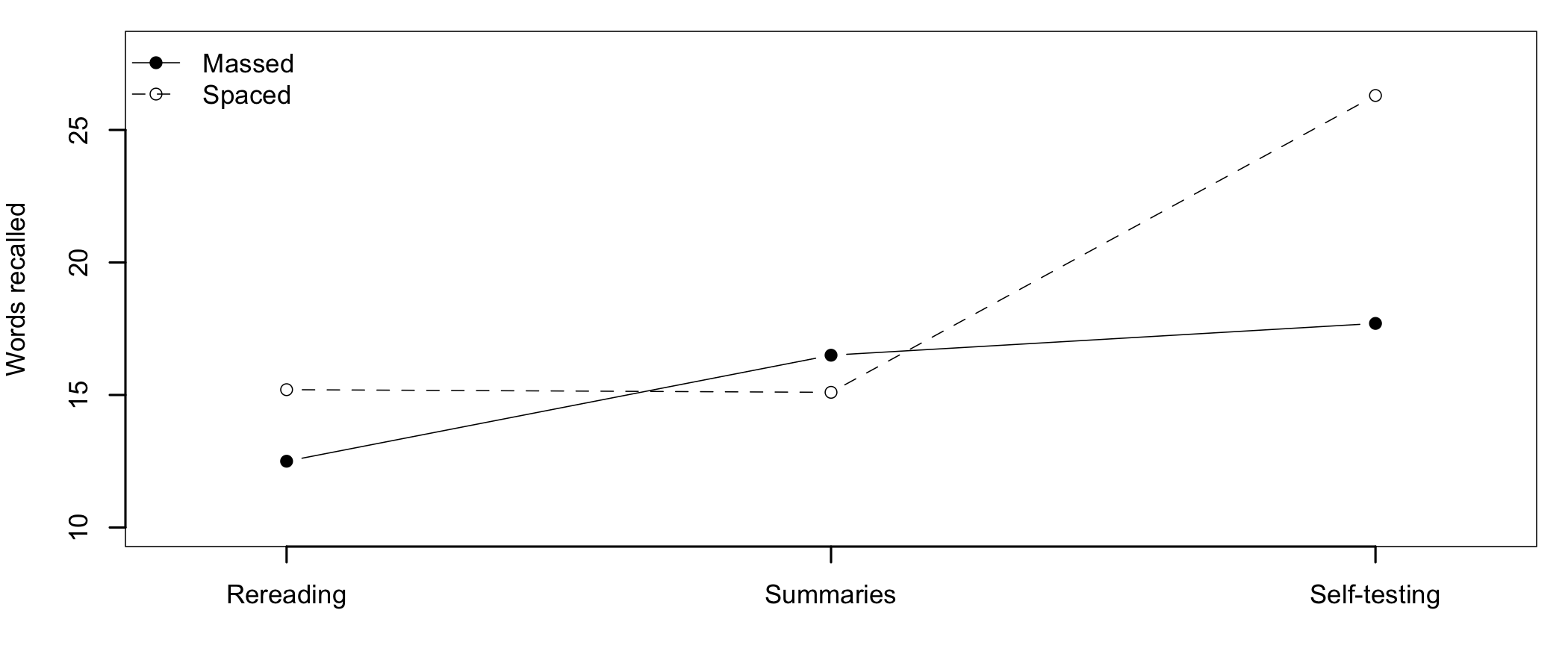
Table 13.3 and Figure 13.2 show that self-testing led to the best recall, especially when the practice was spaced. The students who tested themselves in three short sessions recalled, on average, 26.3 words, compared with 17.7 for those who did it in one session. For the two other methods, the schedule made a much smaller difference, and for the summaries it even went in the other direction. The lines in Figure 13.2 are not parallel, a first sign of an interaction.
13.4.2 Checking the Assumptions
The independence of observations is supported by the design: each student was randomly assigned to one cell and practiced on their own.
                 Massed    Spaced
Rereading    0.67167111 0.8955383
Summaries    0.06436771 0.7761932
Self-testing 0.21302340 0.9396016
Levene's Test for Homogeneity of Variance (center = mean)
Df F value Pr(>F)
group 5 0.9071 0.4834
54 - Normality. The Shapiro-Wilk test is not significant in any of the six cells (p-values between .064 and .940). There is no evidence of a departure from normality in any cell.
- Homogeneity of variances. Levene’s test across the six cells is not significant, F(5, 54) = 0.91, p = .483.
All assumptions are met, so we can proceed with the analysis.
13.4.3 The Two-Way ANOVA
Anova Table (Type III tests)

Response: recall
                 Sum Sq Df  F value    Pr(>F)
(Intercept)     17784.8  1 1645.332 < 2.2e-16 ***
schedule          163.4  1   15.112 0.0002794 ***
method            724.4  2   33.510 3.448e-10 ***
schedule:method   252.7  2   11.689 6.053e-05 ***
Residuals         583.7 54
---
Signif. codes:  0 '***' 0.001 '**' 0.01 '*' 0.05 '.' 0.1 ' ' 1
The output lists one row for each effect88 The (Intercept) row tests whether the grand mean is zero, which is of no interest here.. All three effects are significant:
8 The (Intercept) row tests whether the grand mean is zero, which is of no interest here.
- Schedule: F(1, 54) = 15.11, p < .001, \eta^{2}_{p} = .22;
- Method: F(2, 54) = 33.51, p < .001, \eta^{2}_{p} = .55;
- Schedule \times method: F(2, 54) = 11.69, p < .001, \eta^{2}_{p} = .30.
Decision. The null hypotheses of the two main effects and of the interaction are rejected. Because the interaction is significant, the main effects cannot be taken at face value. The main effect of the schedule, for example, states that spaced practice led to better recall on average, but Figure 13.2 suggests that this is true only for some of the methods.
Effect size. All three effects are large (\eta^{2}_{p} > .14). The method of practice has the largest effect, explaining 55% of the variability that is not explained by the other effects.
13.4.4 Simple Effects
A significant interaction is followed up with simple effects: the effect of one factor at each level of the other factor. The choice of the factor depends on the question asked. Here, the instructor wanted to know for which methods does spacing the practice help? The effect of the schedule is therefore tested separately for each method99 The tests use the error term of the full model, MS_{R}, with 54 degrees of freedom.. Because three tests are run, their p-values are adjusted with the Bonferroni correction.
9 The tests use the error term of the full model, MS_{R}, with 54 degrees of freedom.
 contrast        method       estimate   SE df t.ratio p.value
 Massed - Spaced Rereading        -2.7 1.47 54  -1.836  0.2154
 Massed - Spaced Summaries         1.4 1.47 54   0.952  1.0000
 Massed - Spaced Self-testing     -8.6 1.47 54  -5.849 <0.0001

P value adjustment: bonferroni method for 3 tests
Decision. Spacing the practice improved recall significantly only for self-testing, by 8.6 words, t(54) = 5.85, p < .001. For rereading (a difference of 2.7 words, t(54) = 1.84, p = .215) and for summaries (-1.4 words, t(54) = -0.95, p = 1.000), the differences between the two schedules were small and not significant.
The same interaction can also be read the other way, comparing the methods within each schedule. Both readings describe the same data, and the one reported should answer the question of the study.
schedule = Massed:
 contrast                   estimate   SE df t.ratio p.value
 Rereading - Summaries          -4.0 1.47 54  -2.720  0.0234
 Rereading - (Self-testing)     -5.2 1.47 54  -3.537  0.0024
 Summaries - (Self-testing)     -1.2 1.47 54  -0.816  0.6947

schedule = Spaced:
 contrast                   estimate   SE df t.ratio p.value
 Rereading - Summaries           0.1 1.47 54   0.068  0.9975
 Rereading - (Self-testing)    -11.1 1.47 54  -7.549 <0.0001
 Summaries - (Self-testing)    -11.2 1.47 54  -7.617 <0.0001

P value adjustment: tukey method for comparing a family of 3 estimates
With massed practice, both summaries and self-testing were better than rereading, and did not differ from each other. With spaced practice, self-testing was better than both other methods, which did not differ.
13.4.5 Reporting the Results
| Source | df | SS | MS | F | p | η2p |
|---|---|---|---|---|---|---|
| Schedule | 1 | 163.35 | 163.35 | 15.11 | < .001 | .22 |
| Method | 2 | 724.43 | 362.22 | 33.51 | < .001 | .55 |
| Schedule × Method | 2 | 252.70 | 126.35 | 11.69 | < .001 | .30 |
| Residuals | 54 | 583.70 | 10.81 |
Here is an example of how to write up the results in a publication, together with Table 13.4.
A 2 (schedule: massed, spaced) × 3 (method: rereading, summaries, self-testing) between-subjects ANOVA was conducted on the number of words recalled after a week. The recall scores did not depart significantly from normality in any cell (Shapiro-Wilk p-values between .064 and .940), and the variances were equal (Levene’s test p = .483). There were significant main effects of schedule, F(1, 54) = 15.11, p < .001, η2p = .22, and of method, F(2, 54) = 33.51, p < .001, η2p = .55, qualified by a significant interaction, F(2, 54) = 11.69, p < .001, η2p = .30. Simple effects with a Bonferroni correction showed that spaced practice improved recall for self-testing (M = 26.30 vs. M = 17.70), t(54) = 5.85, p < .001, but not for rereading or summaries (both p > .05).
13.5 Interactions in Regression
At a glance
- Question
- Does the relationship between a predictor and the criterion depend on a second predictor (moderation)?
- Design
- Correlational or experimental, with at least one continuous predictor
- Criterion
- Interval or ratio
- Predictors
- Two, continuous or categorical, and their product (the interaction term)
- Assumptions
-
- The assumptions of multiple regression
- Continuous predictors mean-centered, so their coefficients can be read at the average
- Null hypothesis
- The coefficient of the interaction term is zero
- Test statistic
- t for the interaction coefficient, or F for the change in R2
- Effect size
- \Delta R^{2}, the variance the interaction adds
- If conditions fail
-
- The interaction is significant → Simple slopes: the slope of one predictor at chosen values of the other
- Include in the write-up
-
- Whether the predictors were centered
- The interaction coefficient: b = …, t(df) = …, p = …
- The simple slopes, and R2 with \\Delta R^{2}
The factorial ANOVA requires categorical independent variables. When one or both variables are measured on a continuous scale, the interaction is tested with a regression model that includes the product of the two predictors1010 See Multiple Linear Regression for regression models with several predictors.. With two predictors, X and Z:
10 See Multiple Linear Regression for regression models with several predictors.
\hat{Y} = b_0 + b_1 X + b_2 Z + b_3 XZ
Rearranging the terms shows what the product does:
\hat{Y} = (b_0 + b_2 Z) + (b_1 + b_3 Z)X
The slope of X is no longer a single number, b_1, but b_1 + b_3 Z: it changes with the value of Z. The coefficient of the product, b_3, is the interaction. It shows by how much the slope of X changes for each one-unit increase in Z. If b_3 is zero, the slope is the same for all values of Z and there is no interaction.
Of note is the fact that, in a model with an interaction, b_1 is the slope of X when Z is zero, and b_2 is the effect of Z when X is zero. They are no longer main effects. When zero is not a meaningful value of the predictors, these coefficients are hard to interpret, which is why continuous predictors are usually centered before the analysis1111 Centering subtracts the mean from each value, so that zero becomes the mean. See Mean Centering..
11 Centering subtracts the mean from each value, so that zero becomes the mean. See Mean Centering.
13.5.1 The Study
At the end of the semester, 120 students in a large introductory course reported how many hours per week they had studied for the course, whether they had usually studied alone or in a study group, and how many hours per week they worked at a paid job. The question asked is: Does the benefit of studying depend on how students study and on how much they work? The data set1212 Column labels are: student, mode (Alone or Group), hours, work, and exam. was made up for this example.
12 Column labels are: student, mode (Alone or Group), hours, work, and exam.
    mode        hours             work            exam
 Alone:65   Min.   : 1.100   Min.   : 0.00   Min.   : 39.00
 Group:55   1st Qu.: 7.875   1st Qu.: 8.00   1st Qu.: 60.00
            Median : 9.800   Median :12.00   Median : 65.50
            Mean   : 9.976   Mean   :12.23   Mean   : 65.92
            3rd Qu.:12.025   3rd Qu.:17.00   3rd Qu.: 71.00
            Max.   :21.000   Max.   :27.00   Max.   :100.00
13.5.2 Continuous by Categorical
The first question is whether the relationship between the weekly study hours and the exam score is the same for students who study alone and for those who study in a group. Let’s center the study hours first, so that zero represents a student who studies the average number of hours.
Analysis of Variance Table

Model 1: exam ~ hours.c + mode
Model 2: exam ~ hours.c * mode
  Res.Df    RSS Df Sum of Sq      F   Pr(>F)
1    117 6553.2
2    116 6006.8  1    546.44 10.553 0.001518 **
---
Signif. codes:  0 '***' 0.001 '**' 0.01 '*' 0.05 '.' 0.1 ' ' 1
Hypotheses. H0: In the population, the slope of the study hours is the same for both study modes (b_3 = 0). H1: The slope differs between the two modes (b_3 \neq 0).
Decision criteria. \alpha = .05. The interaction is tested by comparing the model without it (additive model) with the model that includes it (interactive model). H0 is rejected if the p-value of the comparison is smaller than \alpha. The effect size is the increase in R^2 brought by the interaction (\Delta R^2).
Decision. Adding the interaction improved the model significantly, F(1, 116) = 10.55, p = .002. H0 is rejected: the relationship between study hours and the exam score depends on the study mode.
Effect size. The interaction increased R^2 from 0.61 to 0.64, \Delta R^2 = 0.032. It explains about 3% of the variance of the exam scores on top of the two predictors.
Call:
lm(formula = exam ~ hours.c * mode, data = sh)

Residuals:
     Min       1Q   Median       3Q      Max
-22.0127  -4.6388   0.2202   5.2737  15.8120

Coefficients:
                  Estimate Std. Error t value Pr(>|t|)
(Intercept)        65.3323     0.9033  72.326  < 2e-16 ***
hours.c             1.8763     0.2506   7.488 1.49e-11 ***
modeGroup           0.5210     1.3358   0.390  0.69722
hours.c:modeGroup   1.1509     0.3543   3.248  0.00152 **
---
Signif. codes:  0 '***' 0.001 '**' 0.01 '*' 0.05 '.' 0.1 ' ' 1

Residual standard error: 7.196 on 116 degrees of freedom
Multiple R-squared:  0.6435,    Adjusted R-squared:  0.6343
F-statistic: 69.79 on 3 and 116 DF,  p-value: < 2.2e-16
With one categorical predictor coded 0 (Alone) and 1 (Group), the coefficients of the interactive model read:
- Intercept, 65.33: the predicted score of a student who studies alone, for the average number of hours;
- hours.c, 1.88: the slope of the study hours for the students who study alone. Each additional hour adds about 1.9 points;
- modeGroup, 0.52: the difference between studying in a group and studying alone, for the average number of hours;
- hours.c:modeGroup, 1.15: the difference between the two slopes. For the students who study in a group, each additional hour adds 1.15 points more than for those who study alone.
The slopes of the two groups, called simple slopes, can be computed from the coefficients or requested directly:
 mode  hours.c.trend    SE  df t.ratio p.value
 Alone          1.88 0.251 116   7.488 <0.0001
 Group          3.03 0.250 116  12.087 <0.0001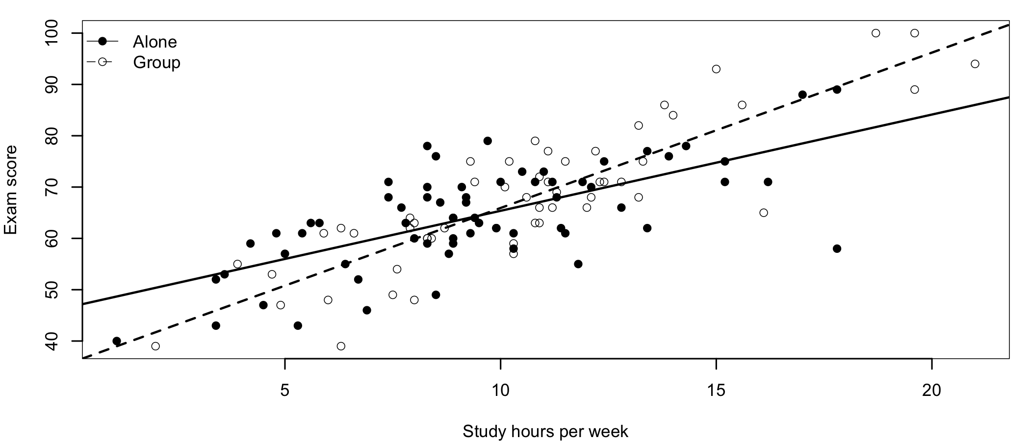
The study hours are a significant predictor of the exam score in both groups, but the line is steeper for the students who study in a group (Figure 13.3): 3.03 points per hour, compared with 1.88 for those who study alone. The lines cross at about 9.5 hours per week. Below this point, the students who study alone have slightly higher predicted scores; above it, those who study in a group do better, and the advantage grows with every additional hour.
Why center? Without centering, the coefficient of modeGroup would be the difference between the two groups for a student who studies zero hours a week, a value outside the range of the data. In the uncentered model it is negative, which could be misread as a disadvantage of group study.
13.5.3 Continuous by Continuous
The second question is whether the benefit of studying depends on how many hours the students work. Both predictors are continuous, and both are centered. The interaction is the product of the two centered variables.
Call:
lm(formula = exam ~ hours.c * work.c, data = sh)

Residuals:
     Min       1Q   Median       3Q      Max
-18.3072  -4.6830   0.7276   5.1132  16.4626

Coefficients:
               Estimate Std. Error t value Pr(>|t|)
(Intercept)    65.63478    0.62732 104.627  < 2e-16 ***
hours.c         2.36106    0.16748  14.098  < 2e-16 ***
work.c         -0.25267    0.09744  -2.593   0.0107 *
hours.c:work.c -0.10328    0.02525  -4.090 7.99e-05 ***
---
Signif. codes:  0 '***' 0.001 '**' 0.01 '*' 0.05 '.' 0.1 ' ' 1

Residual standard error: 6.83 on 116 degrees of freedom
Multiple R-squared:  0.6788,    Adjusted R-squared:  0.6705
F-statistic: 81.72 on 3 and 116 DF,  p-value: < 2.2e-16
Hypotheses. H0: In the population, the slope of the study hours does not change with the hours of work (b_3 = 0). H1: The slope changes with the hours of work.
Decision. The interaction is significant, b_3 = -0.103, t(116) = -4.09, p < .001. H0 is rejected. The negative coefficient means that the slope of the study hours decreases as the hours of work increase: for each additional hour of work per week, an hour of study adds 0.10 points less to the exam score.
Because both predictors are centered, the other coefficients are easy to read. For a student who works the average number of hours (12.2), each hour of study adds 2.36 points. For a student who studies the average number of hours (10.0), each hour of work lowers the exam score by 0.25 points.
With a continuous moderator there are no groups to compare, so the simple slopes are computed at a few representative values of it. A common choice is the mean and one standard deviation below and above it1313 Here, 5.8, 12.2, and 18.7 hours of work per week. Other meaningful values, such as 0, 10, and 20 hours, can be used instead..
13 Here, 5.8, 12.2, and 18.7 hours of work per week. Other meaningful values, such as 0, 10, and 20 hours, can be used instead.
 work.c hours.c.trend    SE  df t.ratio p.value
  -6.48          3.03 0.225 116  13.446 <0.0001
   0.00          2.36 0.167 116  14.098 <0.0001
   6.48          1.69 0.243 116   6.978 <0.0001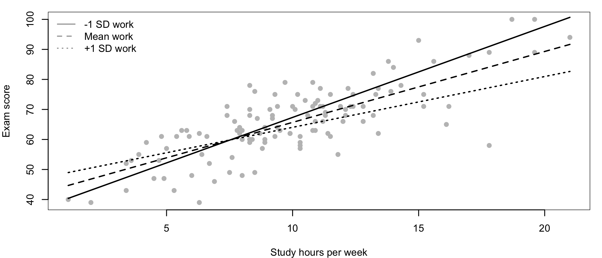
Studying pays off for all students, but less for those who work long hours (Figure 13.4). For a student who works about 6 hours per week, each hour of study adds 3.03 points to the exam score. For a student who works about 19 hours, it adds only 1.69 points1414 A possible explanation is that the students who work long hours study when they are tired. The data cannot tell, and other explanations are possible..
14 A possible explanation is that the students who work long hours study when they are tired. The data cannot tell, and other explanations are possible.
A multiple regression tested whether the hours of paid work moderated the relationship between weekly study hours and exam scores in 120 students. Both predictors were mean-centered. The interaction was significant, b = -0.103, t(116) = -4.09, p < .001. Simple slopes showed that study hours predicted higher exam scores for students who worked one standard deviation below the mean, b = 3.03, p < .001, and one standard deviation above the mean, b = 1.69, p < .001, but the relationship was weaker for students who worked more. The model explained 68% of the variance in exam scores, R2 = .68.
13.6 Summary
A factorial design studies two or more factors at once, and its most important result is the interaction: whether the effect of one factor depends on the level of the other. In the vocabulary study, self-testing was the best practice method, and spacing the practice helped, but only for self-testing. Neither main effect alone tells this story, which is why a significant interaction is interpreted before the main effects, using an interaction plot and simple effects.
The same idea applies to continuous predictors, through the product of the predictors in a regression model. Its coefficient shows by how much the slope of one predictor changes with the other, and the simple slopes show the relationship at meaningful values of the moderator. Centering the continuous predictors before the analysis keeps all coefficients of the model interpretable.