25 Path Analysis
At a glance
- Question
- Does a causal model of several variables fit the data, and how strong are its paths?
- Design
- A causal model with several variables, some of which affect others directly and indirectly
- Variables
- Interval or ratio (observed variables)
- Assumptions
-
- The model is correctly specified (causal order, no missing common causes)
- The variables are measured without error
- The disturbances are uncorrelated
- Null hypothesis
- For the model: it reproduces the observed correlations; for each path, a coefficient of zero
- Test statistic
- The model \chi^{2} and fit indices; z for each path
- Effect size
- The standardized path coefficients (\beta); the indirect and total effects; R2 of each endogenous variable
- Include in the write-up
-
- The model fit: \chi^{2}(df) = …, p = …, CFI, RMSEA, SRMR
- The path coefficients, and the indirect effects with their bootstrap CIs
- The variance explained in the main outcome
Used to test a causal model that links several variables through a network of direct and indirect effects. Path analysis extends mediation analysis, which has one predictor, one mediator, and one criterion, to models with several variables in a chain of causes and effects. The model is drawn as a path diagram and estimated with a set of regressions, one for each variable that receives an arrow, or with a single structural equation model.
Like mediation, path analysis does not discover causes. The researcher draws the model from theory and previous research, and the analysis tests whether the data is consistent with it. The arrows state what causes what and, just as importantly, the missing arrows state which variables do not affect each other directly. A model that fits the data is not proven, because other models, with arrows in other directions, may fit it equally well. A model that does not fit the data, however, can be rejected11 This is why path analysis is described as testing a model by trying to disconfirm it. See also Multiple Linear Regression and A Few Words About Causality..
1 This is why path analysis is described as testing a model by trying to disconfirm it. See also Multiple Linear Regression and A Few Words About Causality.
25.1 The Theory
25.1.1 Path Diagrams
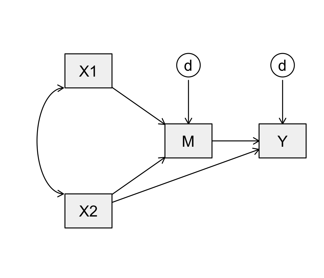
A path diagram shows the variables as boxes and the relationships between them as arrows (Figure 25.1):
- A one-headed arrow is a path, a direct causal effect of one variable on another;
- A curved, two-headed arrow is a correlation that the model does not explain, typically between two variables that are causes in the model;
- A variable that receives no arrows is exogenous: its causes are outside the model. A variable that receives one or more arrows is endogenous: the model explains it, at least in part;
- Each endogenous variable has a disturbance (also called the error or residual term), the part of its variance the model does not explain, due to all its other causes and to measurement error.
The models discussed in this chapter are recursive: the arrows flow in one direction, and no variable can affect itself through a loop. Recursive models can be estimated with ordinary regression.
25.1.2 Direct, Indirect, and Total Effects
A variable can affect another directly, through a path between them, and indirectly, through one or more variables in between. As in mediation, an indirect effect is the product of the paths along its route, and the total effect is the sum of the direct effect and of all the indirect effects22 With standardized coefficients, the effects are expressed in standard deviations, and can be compared across the variables of the model..
2 With standardized coefficients, the effects are expressed in standard deviations, and can be compared across the variables of the model.
25.1.3 Decomposing Correlations
A path model also explains why two variables are correlated. The correlation between two variables in the model can be divided into parts, by following all the routes that connect them in the diagram33 The routes are found with tracing rules: a route can go backward along arrows and then forward, but not forward and then backward; it cannot pass through the same variable twice; and it can include at most one two-headed arrow. The rules were introduced by the geneticist Sewall Wright in the 1920s.:
3 The routes are found with tracing rules: a route can go backward along arrows and then forward, but not forward and then backward; it cannot pass through the same variable twice; and it can include at most one two-headed arrow. The rules were introduced by the geneticist Sewall Wright in the 1920s.
- Direct effect, the path from one variable to the other;
- Indirect effects, the routes from one variable to the other through other variables, always following the direction of the arrows;
- Spurious effects, the routes through a common cause of both variables. They create a correlation without any causal effect between the two variables;
- Unanalyzed effects, the routes through a correlation between exogenous variables, which the model does not explain.
Only the first two are causal. The difference between a correlation and the total effect shows how much of the relationship is due to common causes, and how wrong it would be to read the correlation as an effect.
25.1.4 Estimating the Model
There are two ways of estimating a recursive path model:
- With a set of regressions. Each endogenous variable is regressed on the variables that have arrows pointing to it. The standardized slopes are the path coefficients, and the disturbance of each endogenous variable is \sqrt{1 - R^2}, the standard deviation of its unexplained part;
- With structural equation modeling (SEM), which estimates all paths at once. The coefficients are the same, but SEM also tests the fit of the whole model and computes the indirect effects and their standard errors.
25.1.5 Model Fit
A model with an arrow, or a correlation, between every pair of variables is saturated: it reproduces the observed correlations exactly, and its fit cannot be tested. Every missing arrow is a restriction, a statement that the direct effect is zero, and gives the model one degree of freedom. A model with degrees of freedom predicts some correlations that it does not reproduce exactly, and the fit of the model measures how close these predictions are to the observed correlations. The most common fit measures are44 The thresholds below are rules of thumb: for the CFI, the RMSEA, and the SRMR from Hu and Bentler (1999), and for a poor RMSEA from Browne and Cudeck (1993).:
- The chi-square test. Its null hypothesis is that the model fits the data perfectly, so a non-significant chi-square is the desired result55 With large samples, the test rejects even models with small and unimportant misfit.;
5 With large samples, the test rejects even models with small and unimportant misfit.
- The Comparative Fit Index (CFI), which compares the model with a model in which all variables are uncorrelated. Values of .95 or more indicate a good fit;
- The Root Mean Square Error of Approximation (RMSEA), which measures the misfit per degree of freedom. Values of .06 or less indicate a good fit, and values above .10 a poor one;
- The Standardized Root Mean Square Residual (SRMR), the average difference between the observed and the predicted correlations. Values of .08 or less indicate a good fit.
A model should be judged on several measures together, and on how well it agrees with theory.
25.2 Assumptions
Path analysis has the assumptions of multiple regression for each equation of the model: linear relationships, independent observations, normally distributed residuals, and no extreme multicollinearity. It also has the causal assumptions discussed for mediation:
- The model is correctly specified: the causal order of the variables is right, and no important common cause is missing;
- The variables are measured without error, especially the exogenous variables. Measurement error biases the path coefficients, usually toward zero66 Models with latent variables, measured by several indicators, take measurement error into account. They are part of structural equation modeling.;
6 Models with latent variables, measured by several indicators, take measurement error into account. They are part of structural equation modeling.
- The disturbances are uncorrelated with each other and with the variables that cause the endogenous variable they belong to77 A correlated disturbance means that a common cause has been left out..
7 A correlated disturbance means that a common cause has been left out.
25.3 The Study
A university’s first-year program wanted to understand how students’ backgrounds and beliefs lead to their grades at the end of the first year. Based on research on academic success, the program staff proposed the model in Figure 25.2:
- Family support and high school GPA, measured when the students arrived, are the exogenous variables. They are allowed to be correlated;
- Both affect the students’ self-efficacy88 The students’ confidence that they can succeed in their courses., measured at mid-year;
8 The students’ confidence that they can succeed in their courses.
- Self-efficacy affects engagement99 The number of hours per week the students spent studying., also measured at mid-year;
9 The number of hours per week the students spent studying.
- The first-year grade average depends on high school GPA, self-efficacy, and engagement.
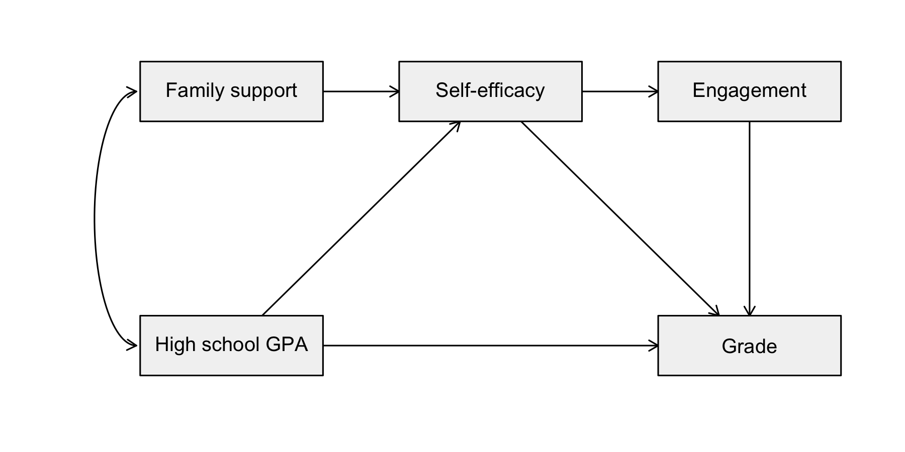
The missing arrows are part of the model. Family support is expected to affect engagement and grades only through self-efficacy, and high school GPA to affect engagement only through self-efficacy. The model has three missing arrows, and therefore three degrees of freedom to test its fit.
Three hundred students took part in the study. The data set1010 Column labels are: student, support, hsgpa, efficacy, engagement, and grade. was made up for this example. The first few rows of the data set are shown in Table 25.1.
10 Column labels are: student, support, hsgpa, efficacy, engagement, and grade.
| Student | Support | HS GPA | Self-efficacy | Engagement | Grade |
|---|---|---|---|---|---|
| 1 | 2.7 | 2.76 | 35 | 6.1 | 54 |
| 2 | 3.4 | 3.23 | 32 | 5.4 | 75 |
| 3 | 3.2 | 3.68 | 29 | 6.6 | 79 |
| 4 | 4.5 | 3.34 | 45 | 22.6 | 71 |
| 5 | 4.9 | 4.00 | 50 | 22.4 | 86 |
| 6 | 2.5 | 2.79 | 26 | 7.8 | 72 |
| Support | HS GPA | Self-efficacy | Engagement | |
|---|---|---|---|---|
| Support | ||||
| HS GPA | .19 | |||
| Self-efficacy | .48 | .37 | ||
| Engagement | .27 | .19 | .41 | |
| Grade | .18 | .52 | .44 | .43 |
All variables are positively correlated (Table 25.2). The model will explain these correlations as direct, indirect, and spurious effects.
Hypotheses. A path analysis tests the model as a whole and each of its paths:
- Model fit. H0: The model reproduces the correlations in the population. H1: It does not.
- Each path. H0: In the population, the direct effect is zero. H1: It is different from zero.
- Each indirect effect of interest. H0: In the population, the indirect effect is zero. H1: It is different from zero.
Decision criteria. The significance level is set at \alpha = .05. The model is retained if the chi-square test is not significant and the fit measures are in their recommended ranges. The paths are tested with z tests, and the indirect effects with 95% bootstrap confidence intervals.
25.3.1 The Model as a Set of Regressions
Each endogenous variable is regressed on its causes, as specified by the arrows. To obtain the path coefficients directly, the variables are standardized first.
(Intercept)     support       hsgpa
      0.000       0.424       0.294
(Intercept) efficacy
0.000 0.407 (Intercept) hsgpa efficacy engagement
0.000 0.405 0.171 0.284 efficacy engagement grade
0.829 0.913 0.770 Each slope is the direct effect of a cause on its effect, holding the other causes of the same variable constant. The disturbances show how much of each endogenous variable is left unexplained. The grades, for example, have a disturbance of 0.77, which means that the model explains 1 - 0.77^2 = 0.41 of their variance. The regressions estimate the paths, but they do not test the model as a whole. For that, the model is estimated as a structural equation model.
25.3.2 The Model as a Structural Equation Model
lavaan 0.6-21 ended normally after 15 iterations

  Estimator                                         ML
  Optimization method                           NLMINB
  Number of model parameters                        12

  Number of observations                           300

Model Test User Model:

  Test statistic                                 5.112
  Degrees of freedom                                 3
  P-value (Chi-square)                           0.164

Model Test Baseline Model:

  Test statistic                               339.613
  Degrees of freedom                                10
  P-value                                        0.000

User Model versus Baseline Model:

  Comparative Fit Index (CFI)                    0.994
  Tucker-Lewis Index (TLI)                       0.979

Loglikelihood and Information Criteria:

  Loglikelihood user model (H0)              -3277.404
  Loglikelihood unrestricted model (H1)      -3274.848

  Akaike (AIC)                                6578.808
  Bayesian (BIC)                              6623.253
  Sample-size adjusted Bayesian (SABIC)       6585.196

Root Mean Square Error of Approximation:

  RMSEA                                          0.048
  90 Percent confidence interval - lower         0.000
  90 Percent confidence interval - upper         0.118
  P-value H_0: RMSEA <= 0.050                    0.422
  P-value H_0: RMSEA >= 0.080                    0.280

Standardized Root Mean Square Residual:

  SRMR                                           0.023

Parameter Estimates:

  Standard errors                            Bootstrap
  Number of requested bootstrap draws             2000
  Number of successful bootstrap draws            2000

Regressions:
                   Estimate  Std.Err  z-value  P(>|z|)   Std.lv  Std.all
  efficacy ~
    support   (a1)    3.984    0.423    9.417    0.000    3.984    0.424
    hsgpa     (a2)    5.025    0.805    6.245    0.000    5.025    0.294
  engagement ~
    efficacy  (b1)    0.296    0.035    8.415    0.000    0.296    0.407
  grade ~
    hsgpa     (c1)    8.054    0.870    9.256    0.000    8.054    0.406
    efficacy  (c2)    0.199    0.059    3.343    0.001    0.199    0.171
    engagemnt (c3)    0.455    0.076    6.004    0.000    0.455    0.285

Covariances:
                   Estimate  Std.Err  z-value  P(>|z|)   Std.lv  Std.all
  support ~~
    hsgpa             0.055    0.018    3.068    0.002    0.055    0.188

Variances:
                   Estimate  Std.Err  z-value  P(>|z|)   Std.lv  Std.all
   .efficacy         32.370    2.349   13.782    0.000   32.370    0.687
   .engagement       20.779    1.679   12.374    0.000   20.779    0.834
   .grade            37.973    2.864   13.261    0.000   37.973    0.598
    support           0.533    0.038   14.206    0.000    0.533    1.000
    hsgpa             0.162    0.013   12.386    0.000    0.162    1.000

Defined Parameters:
                   Estimate  Std.Err  z-value  P(>|z|)   Std.lv  Std.all
    eff_grade         0.135    0.028    4.783    0.000    0.135    0.116
    sup_grade         1.329    0.262    5.069    0.000    1.329    0.122
    gpa_grade         1.676    0.424    3.950    0.000    1.676    0.085
Decision (model fit). The chi-square test is not significant, \chi^{2}(3) = 5.11, p = .164: the model’s predictions do not differ significantly from the observed correlations. The other fit measures agree: CFI = 0.994, RMSEA = 0.048 (90% CI from 0.000 to 0.118), and SRMR = 0.023. The model is retained.
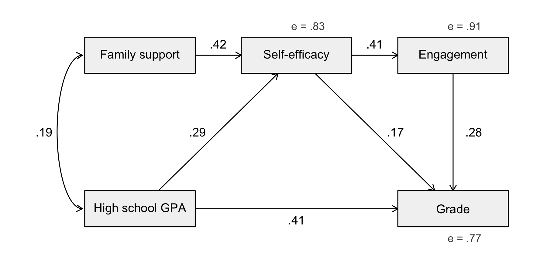
Decision (paths). All six paths are significant (Figure 25.3)1111 The Std.all column of the output shows the standardized coefficients, the same values as the regressions of standardized variables.:
11 The Std.all column of the output shows the standardized coefficients, the same values as the regressions of standardized variables.
- Self-efficacy is higher for students with more family support (\beta = .42, z = 9.42, p < .001) and a higher high school GPA (\beta = .29, z = 6.25, p < .001);
- Students with higher self-efficacy are more engaged (\beta = .41, z = 8.42, p < .001);
- The first-year grade depends most on high school GPA (\beta = .41, z = 9.26, p < .001), then on engagement (\beta = .28, z = 6.00, p < .001), and on self-efficacy (\beta = .17, z = 3.34, p < .001).
25.3.3 Indirect and Total Effects
The defined parameters at the end of the output are the indirect effects on the grade, in raw units, with bootstrap confidence intervals:
- Self-efficacy affects the grade indirectly, through engagement, b = 0.135, 95% CI [0.084, 0.195], \beta = .12;
- Family support has no direct effect on the grade in the model, but affects it indirectly, through self-efficacy and engagement, b = 1.329, 95% CI [0.830, 1.844], \beta = .12;
- High school GPA affects the grade directly and also indirectly, through self-efficacy and engagement, b = 1.676, 95% CI [0.927, 2.578], \beta = .08.
The unstandardized indirect effects (b) are in grade points1212 One more point of self-efficacy, for example, raises the grade by 0.135 points through its effect on engagement.. None of the confidence intervals includes zero: all three indirect effects are significant.
12 One more point of self-efficacy, for example, raises the grade by 0.135 points through its effect on engagement.
Let’s now decompose the correlation between self-efficacy and the grade, r = 0.44, using the standardized coefficients:
| Component | Value |
|---|---|
| Direct effect (self-efficacy → grade) | 0.171 |
| Indirect effect (through engagement) | 0.116 |
| Total effect | 0.287 |
| Spurious (common causes: support, high school GPA) | 0.150 |
| Correlation | 0.437 |
The total causal effect of self-efficacy on the grade is 0.287, of which 40% passes through engagement. The rest of the correlation, 0.150, is spurious: it exists because students with a higher high school GPA and more family support tend to have both a higher self-efficacy and, for other reasons, higher grades. About 34% of the correlation is spurious, and reading the correlation as the effect of self-efficacy would overestimate that effect by 52%.
25.3.4 Comparing Models
Is the model too simple? The three missing paths can be tested by adding them to the model and comparing the two models. The model with all paths is saturated, and the comparison is a chi-square difference test.
Chi-Squared Difference Test

       Df    AIC    BIC  Chisq Chisq diff    RMSEA Df diff Pr(>Chisq)
my.sat  0 6579.7 6635.3 0.0000
my.fit  3 6578.8 6623.3 5.1122     5.1122 0.048444       3     0.1638
The saturated model does not fit the data significantly better, \chi^{2}(3) = 5.11, p = .164, and the proposed model has the lower AIC and BIC. The three additional paths are not needed: the simpler model, which states that family support affects engagement and grades only through self-efficacy, is preferred1313 See Occam’s Razor..
13 See Occam’s Razor.
25.3.5 Reporting the Results
A path analysis tested a model of first-year grades in which family support and high school GPA affected academic self-efficacy, self-efficacy affected engagement, and the first-year grade depended on high school GPA, self-efficacy, and engagement (N = 300). The model fit the data well, χ2(3) = 5.11, p = .164, CFI = .994, RMSEA = .048, SRMR = .023, and did not fit significantly worse than a saturated model, p = .164. All paths were significant (Figure 25.3). The strongest predictor of the first-year grade was high school GPA (β = .41), followed by engagement (β = .28) and self-efficacy (β = .17). Family support affected the grade only indirectly, through self-efficacy and engagement, b = 1.329, 95% bootstrap CI [0.830, 1.844], β = .12. The model explained 41% of the variance in first-year grades.
25.4 Summary
Path analysis tests a causal model that links several variables through direct and indirect effects. The model is drawn from theory, before the data is analyzed, and the analysis estimates its paths and tests whether its missing paths are consistent with the data. In the first-year study, the model fit the data well: family support and high school GPA raised the students’ self-efficacy, self-efficacy raised their engagement, and both led to better grades. The decomposition of the correlations showed how much of the relationship between self-efficacy and grades was causal, and how much was due to common causes.
Of note is the fact that a good fit does not make the model true. Other models, with arrows in other directions, may fit the same correlations equally well, and a common cause left out of the model would bias its paths. The order in which the variables were measured, the theory behind the model, and the comparison with alternative models are what make a path model convincing.